Exploratory data analysis & experimental design

Keegan Korthauer

January 16, 2024

Today: Getting to know your data, and why you need to understand where it came from

Learning objectives:

  1. Understand general principles on organizing your data

  2. Be familiar with the main components of exploratory data analysis (EDA)

  3. Recognize and avoid common pitfalls of data visualization

  4. Understand the impacts of data quality and experimental design

Where to find code to make these plots

Instructions to create .pdfs from the .html slides:

  1. Open slides in Google Chrome or Chromium
  2. Toggle into print view by pressing the E key
  3. Open the print dialogue by pressing: CTRL/CMD+P
  4. Change the Destination setting to Save as PDF
  5. Change the Layout to Landscape
  6. Change the Margins to None
  7. Enable the Background graphics option
  8. Click Save

CHD8 RNA-seq experiment

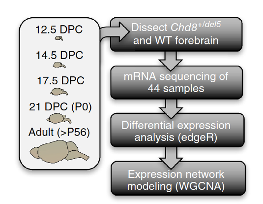
  • Gompers et al. (Nature Neuroscience 2017) performed RNA-seq on mice from two different genotypes (18 WT vs 26 CHD8 mutant) and 5 developmental stages

  • “Using a statistical model that accounted for sex, developmental stage and sequencing batch, we tested for differential expression across 11,936 genes that were robustly expressed”

  • We’ll use this dataset throughout this lecture to illustrate EDA

Data organization

  • As is often the case, this data was obtained in two separate files

    • Main data file: expression values - one per gene, per sample ( \(G\) genes \(\times\) \(N\) samples)

    • Metadata file: several covariates/experimental design variables for each sample ( \(N\) samples \(\times\) \(P\) covariates)

  • We read these into R (see Rmd source code and companion notes) as a data.frame or tibble - matrix-like objects that have column names, and variable types for each column:

# data (expression) matrix
dim(d)
[1] 12158    44
# metadata
dim(m)
[1] 44  8

Small but important detail

Columns of main data matrix should match the rows of the metadata matrix exactly

These two objects should represent the same set of samples (and be in the same order)

head(colnames(d))
[1] "Sample_ANAN001A" "Sample_ANAN001B" "Sample_ANAN001C" "Sample_ANAN001D"
[5] "Sample_ANAN001E" "Sample_ANAN001F"
head(m$Sample)
[1] "Sample_ANAN001A" "Sample_ANAN001B" "Sample_ANAN001C" "Sample_ANAN001D"
[5] "Sample_ANAN001E" "Sample_ANAN001F"
identical(colnames(d), m$Sample)
[1] TRUE

Data matrix

head(d)
              Sample_ANAN001A Sample_ANAN001B Sample_ANAN001C Sample_ANAN001D
0610007P14Rik        5.238647        5.042397        5.364602        5.207641
0610009B22Rik        4.251070        4.568908        4.625527        4.568743
0610009O20Rik        4.807282        4.743503        4.921915        4.813903
0610010F05Rik        4.830067        5.063055        4.861288        4.957009
0610010K14Rik        5.958641        5.810707        5.851939        6.043380
0610011F06Rik        4.619302        4.579443        4.900748        4.802624
              Sample_ANAN001E Sample_ANAN001F Sample_ANAN001G Sample_ANAN001H
0610007P14Rik        5.222326        5.129427        5.239697        5.127338
0610009B22Rik        4.555767        4.412691        4.253776        4.205859
0610009O20Rik        4.812471        4.807076        4.828430        4.708997
0610010F05Rik        5.065935        4.948113        5.067492        5.124294
0610010K14Rik        5.997013        5.979884        5.902530        5.846258
0610011F06Rik        4.756396        4.828523        4.575162        4.868060
              Chd8.e14.S12 Chd8.e14.S13 Chd8.e14.S14 Chd8.e14.S16 Chd8.e14.S17
0610007P14Rik     4.841569     5.197562     4.825154     5.181760     5.070708
0610009B22Rik     4.452122     4.746104     4.747871     4.789378     4.862351
0610009O20Rik     4.455875     4.649412     4.338314     4.555878     4.490673
0610010F05Rik     5.314438     5.387970     5.523043     5.308837     5.514546
0610010K14Rik     5.855191     6.148984     6.148754     6.098012     6.174872
0610011F06Rik     4.391892     4.890393     4.486821     4.836696     4.446990
              Chd8.e14.S18 Chd8.e14.S19 Chd8.e14.S20 Chd8.e14.S21
0610007P14Rik     5.237254     5.283928     5.196948     5.022812
0610009B22Rik     4.871463     5.062306     4.819321     4.719951
0610009O20Rik     4.474563     4.597433     4.578242     4.506912
0610010F05Rik     5.430677     5.185067     5.477901     5.488947
0610010K14Rik     6.253634     6.561689     6.133367     6.032934
0610011F06Rik     4.698659     5.281168     4.785467     4.610248
              Chd8.e17.5.1_S158 Chd8.e17.5.2_S159 Chd8.e17.5.4_S161
0610007P14Rik          5.504698          5.563476          5.469537
0610009B22Rik          3.880660          4.366783          4.187023
0610009O20Rik          4.367506          4.074845          4.016735
0610010F05Rik          5.352970          5.406458          5.437642
0610010K14Rik          6.020094          5.818114          6.029098
0610011F06Rik          4.222639          4.064907          4.237808
              Chd8.e17.5.5_S162 Chd8.e17.5.6_S163 Chd8.e17.5.1_S1
0610007P14Rik          5.210378          5.747802        5.360175
0610009B22Rik          3.896679          4.109132        4.083653
0610009O20Rik          4.260492          4.310498        4.171089
0610010F05Rik          5.270270          5.498813        5.237495
0610010K14Rik          5.830401          6.202582        5.907929
0610011F06Rik          4.255365          4.301042        4.208392
              Chd8.e17.5.2_S2 Chd8.e17.5.3_S3 Chd8.e17.5.4_S4 Chd8.e17.5.5_S5
0610007P14Rik        5.396869        5.480500        5.576968        5.792268
0610009B22Rik        4.012442        4.043540        4.023286        4.115983
0610009O20Rik        4.181214        4.075280        4.243173        4.396101
0610010F05Rik        5.359145        5.590551        5.466983        5.332507
0610010K14Rik        6.142755        6.067490        5.856817        6.354569
0610011F06Rik        4.355365        4.199820        4.108307        4.591746
              Chd8.P0.S1 Chd8.P0.S10 Chd8.P0.S11 Chd8.P0.S2 Chd8.P0.S3
0610007P14Rik   5.004910    5.618407    5.042920   5.516423   5.249834
0610009B22Rik   3.171498    3.817326    3.381746   3.585340   3.481041
0610009O20Rik   4.262572    4.276003    4.245660   4.234671   4.302060
0610010F05Rik   5.063260    5.308997    5.113254   5.273173   5.179340
0610010K14Rik   5.968141    6.273270    5.865349   6.197163   6.144795
0610011F06Rik   3.834333    4.442323    4.143605   4.277508   4.370633
              Chd8.P0.S4 Chd8.P0.S5 Chd8.P0.S6 Chd8.P0.S7 Chd8.P0.S8 Chd8.P0.S9
0610007P14Rik   5.490179   5.330979   5.089818   5.309648   5.207886   5.280196
0610009B22Rik   3.814849   3.634283   3.425465   3.657936   3.647259   3.641667
0610009O20Rik   4.262546   4.112654   4.331208   4.281473   4.390390   4.241503
0610010F05Rik   5.254348   5.272861   5.208265   5.232609   5.102297   5.227704
0610010K14Rik   6.153272   6.076559   6.136792   6.236681   6.217135   6.246569
0610011F06Rik   4.206831   4.138643   4.091530   4.309412   4.398383   4.260990
              Chd8.adult.S23 Chd8.adult.S24 Chd8.adult.S25 Chd8.adult.S28
0610007P14Rik       5.117776       5.105053       5.074071       5.274795
0610009B22Rik       3.736176       4.437970       4.150157       4.726862
0610009O20Rik       4.218049       4.409190       4.386743       4.494319
0610010F05Rik       4.391540       3.700743       3.745234       3.602500
0610010K14Rik       5.245851       4.827066       4.953091       4.971989
0610011F06Rik       4.562028       4.714897       4.696579       5.080126
              Chd8.adult.S29 Chd8.adult.S31
0610007P14Rik       5.051701       5.000228
0610009B22Rik       4.046562       4.485514
0610009O20Rik       4.402777       4.321922
0610010F05Rik       3.715847       3.912299
0610010K14Rik       4.910206       4.861016
0610011F06Rik       4.787186       4.849831

Metadata

m
# A tibble: 44 × 8
   Number Sample            DPC Sex   Group  SeqRun MappedReads FeatureCounts
    <dbl> <chr>           <dbl> <fct> <fct>  <fct>        <dbl>         <dbl>
 1      1 Sample_ANAN001A  12.5 F     Mutant A         42452222      37655856
 2      2 Sample_ANAN001B  12.5 M     WT     A         54503162      47106938
 3      3 Sample_ANAN001C  12.5 M     WT     A         44978512      40448118
 4      4 Sample_ANAN001D  12.5 F     Mutant A         50099336      44993589
 5      5 Sample_ANAN001E  12.5 F     Mutant A         47163546      41840678
 6      6 Sample_ANAN001F  12.5 F     WT     A         43893480      39483622
 7      7 Sample_ANAN001G  12.5 F     Mutant A         53208684      47697298
 8      8 Sample_ANAN001H  12.5 F     WT     A         38925414      35056860
 9      9 Chd8.e14.S12     14.5 M     WT     B         23622816      19586363
10     10 Chd8.e14.S13     14.5 F     WT     B         23974703      21019829
# ℹ 34 more rows

Organizing your data - two main issues

  • How you set up your input files for easy reading into R

    • Easiest to work with are text files (e.g. tab-delimited .tsv)

    • Excel files not uncommon but not recommended

    • Almost always some data cleaning/wrangling involved (e.g. checking consistency, recoding, renaming variables)

  • Within R, being able to refer to subsets of both data sets (main data & metadata) and other manipulations that require “matching” the expression data with the sample information (“slicing and dicing”)

    • For example: “Get me the expression level data for CHD8 in the female adult wild type mice” – this uses information from both sets

    • In practice, you may have to do it multiple ways to play nice with different R packages (e.g. one way for visualization, and another for downstream analysis)

Organizing your data: Separated

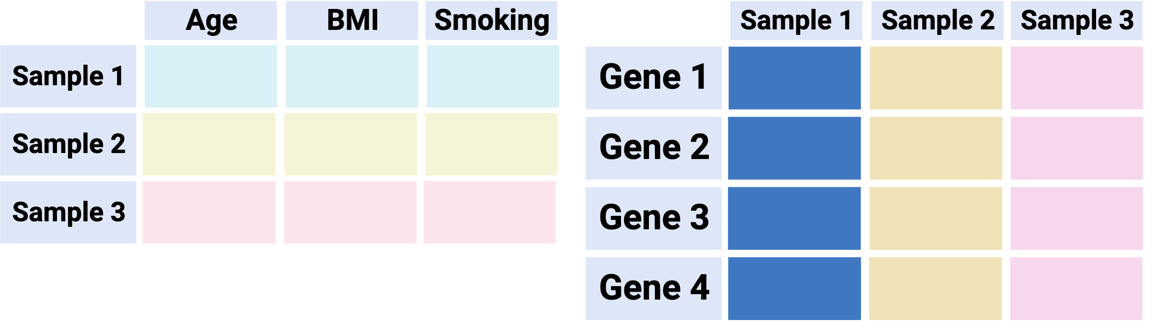
Option 1 - “Separated”: Keep main data and metadata tables separate

Pros:

  • Minimal startup effort / extra code

  • Can be compatible with downstream analysis methods (e.g. Bioconductor)

Cons:

  • Risky: easy to make a mistake when subsetting and/or reordering samples - extra sanity checks required

  • Not a convenient format for visualization since main data is separated from its metadata

Overall: not recommended

Organizing your data: Tidy way

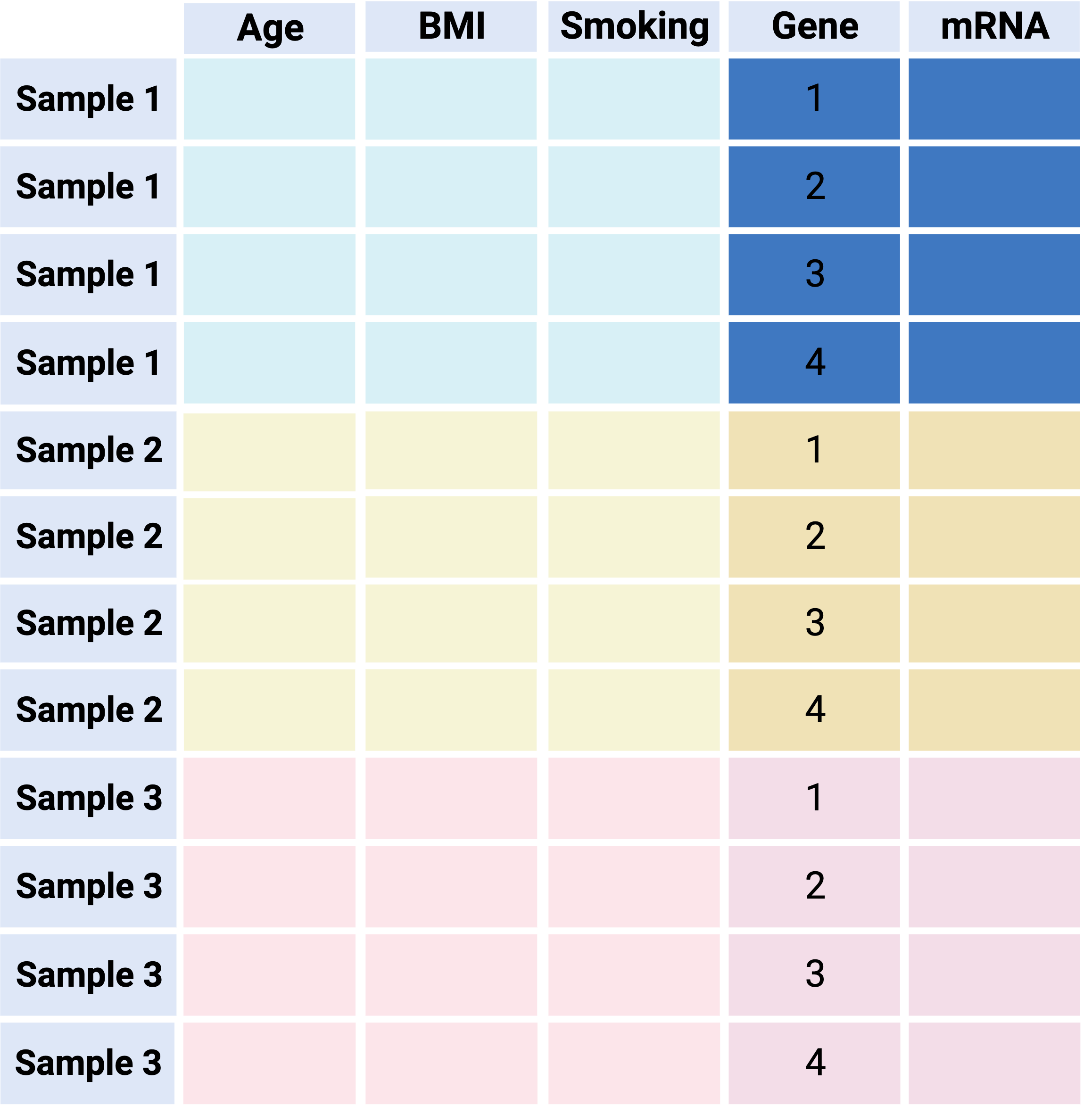
Option 2 - “The tidy way”: Combine main data & metadata into one ‘long’ table

Pros:

  • Unambiguous - keeps all data in one object with one row per observation (e.g. each sample/gene combination is one row, along with all its metadata)

  • Plays nice with tidyverse tools (e.g. dplyr manipulations, ggplot2 visualization)

Cons:

  • ‘long’ format is inefficient data storage - sample information is repeated

  • Not compatible with many tools for downstream analysis (e.g. Bioconductor)

Overall: recommended for EDA/visualization

The Tidy way

d_long
# A tibble: 534,952 × 10
   gene          Sample   Expression Number   DPC Sex   Group SeqRun MappedReads
   <chr>         <chr>         <dbl>  <dbl> <dbl> <fct> <fct> <fct>        <dbl>
 1 0610007P14Rik Sample_…       5.24      1  12.5 F     Muta… A         42452222
 2 0610009B22Rik Sample_…       4.25      1  12.5 F     Muta… A         42452222
 3 0610009O20Rik Sample_…       4.81      1  12.5 F     Muta… A         42452222
 4 0610010F05Rik Sample_…       4.83      1  12.5 F     Muta… A         42452222
 5 0610010K14Rik Sample_…       5.96      1  12.5 F     Muta… A         42452222
 6 0610011F06Rik Sample_…       4.62      1  12.5 F     Muta… A         42452222
 7 0610012G03Rik Sample_…       4.03      1  12.5 F     Muta… A         42452222
 8 0610030E20Rik Sample_…       3.22      1  12.5 F     Muta… A         42452222
 9 0610031J06Rik Sample_…       4.38      1  12.5 F     Muta… A         42452222
10 0610037L13Rik Sample_…       4.23      1  12.5 F     Muta… A         42452222
# ℹ 534,942 more rows
# ℹ 1 more variable: FeatureCounts <dbl>

Organizing data: Bioconductor way

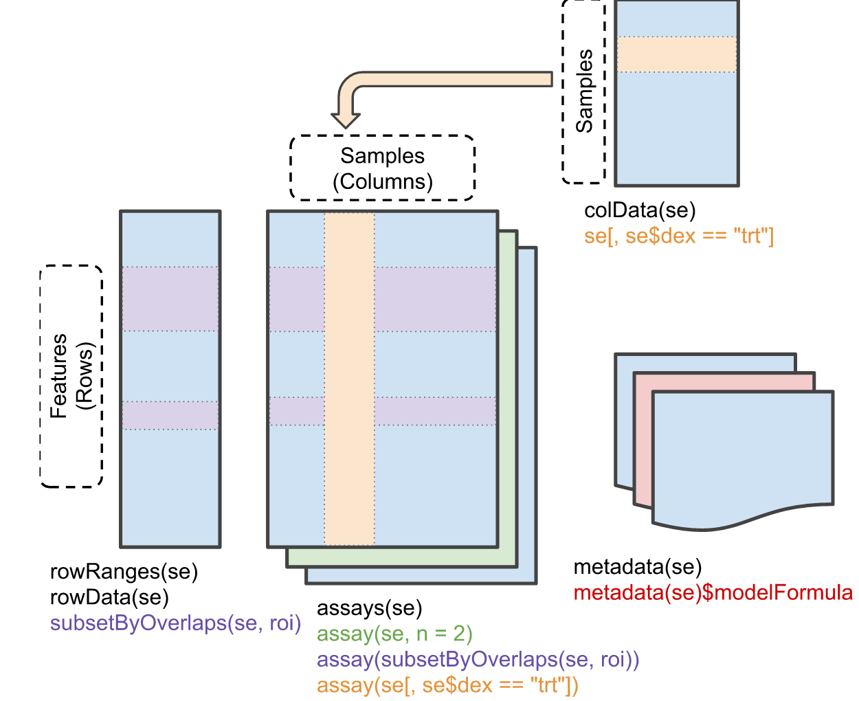
Option 3 - “The Bioconductor way”: Combine main data & metadata into one specially formatted object

Pros:

  • Unambiguous: keeps all data in one object with special slots that can be accessed with handy functions

  • Plays nice with Bioconductor tools

  • Efficient storage (no duplication of information like tidy way)

Cons:

  • Specific to Bioconductor

  • Not a compatible format for visualization (e.g. ggplot2)

Overall: recommended for downstream analysis (e.g. Differential Expression)

The Bioconductor way: SummarizedExperiment

Now what? Time to explore!

  • Understand / get a feel for the data

  • Formulate hypotheses / develop models

  • Identify problems

First questions - sanity checks

  • Is the file the expected size? Format?

  • Do we have the expected number of samples?

  • Do the sample names in both files match? (Do not assume same ordering!)

  • Are sample / feature names formatted correctly (e.g. no Excel conversion errors)?

  • What do features represent? (e.g. Gene names, probe identifiers, etc.)

  • Is the data numeric? Integers or decimal? Ratios (to what?)

  • Are the data on a log scale? If so what is the base?

  • Are there missing data points? What do they mean?

  • Do factors have the expected number of levels?

  • Do we have all the sample information we need?

These questions might lead to concerns

  • If you are the one generating the data, save yourself grief by paying attention to these issues up front - Document what you did and be consistent!

  • If you are the analyst, hopefully you were involved in the design stage so there will be fewer surprises

Making sense of the data

Data is what we observe, we want to infer something about “where it came from”

Model of gene expression data generation

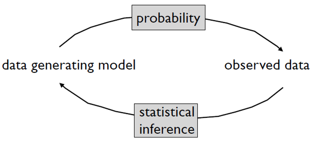
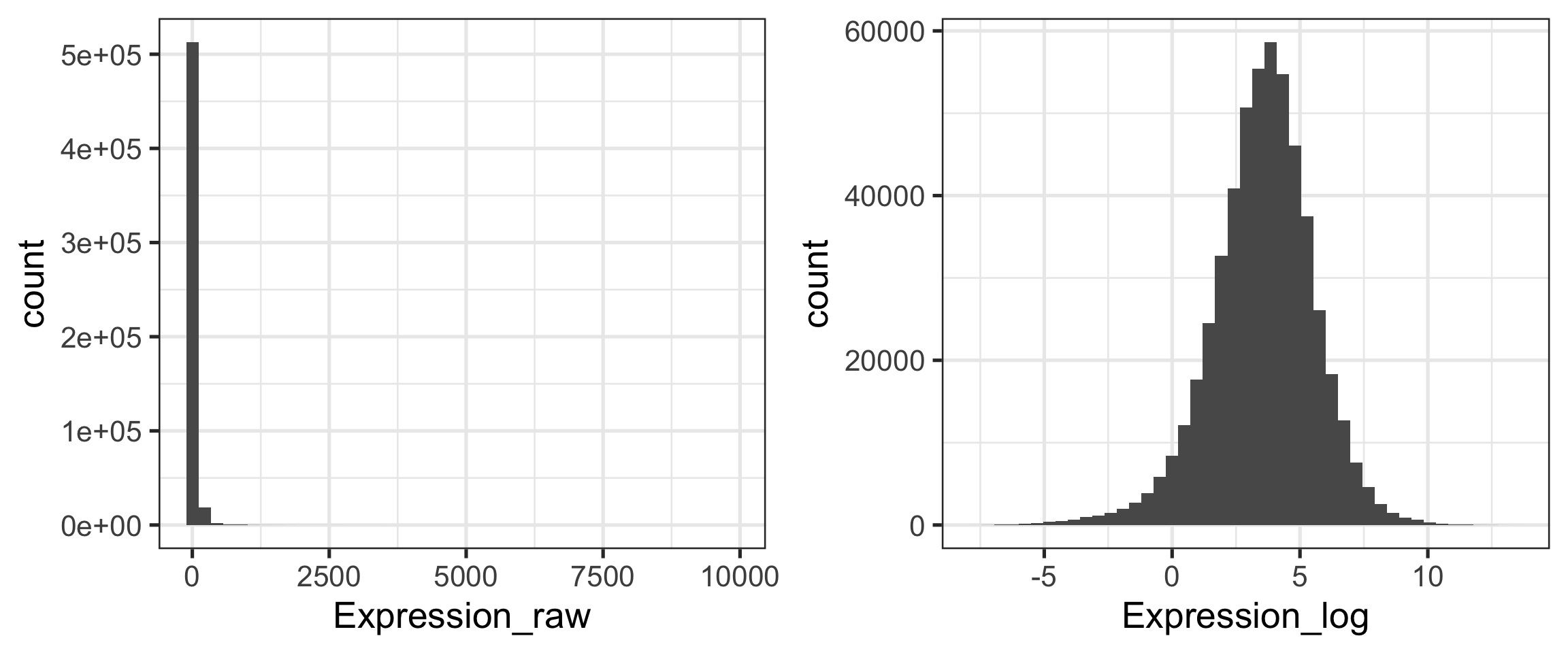
  • The measured expression level of gene \(g\) is the combination of many effects

  • Analysis goal is often to determine relative role of effects - separate signal from “noise”

Variability: friend and foe

  • If there is no variability, you don’t have any information - key is controlling/understanding sources of wanted vs. unwanted variability

  • First line of defense: Know the enemy

    • You can only “correct” for things you know about

    • Keep track of potential sources of variance: Batches of reagents, slides, personnel, processing dates, etc.

  • Design experiments to minimize impact of technical variability

    • Don’t process all control samples on day 1 and all treated samples on day 10
  • Ensure appropriate replication

    • Biological (important)

    • Technical (usually less important but might need to convince yourself)

Biggest pitfall in (high-dimensional) data analysis

If you don’t look at the data, you are likely going to miss important things

  • Not just at the beginning, but at every stage

  • That could mean making plots, or examining numerical patterns - probably both

  • “Sanity checks” should make up a lot of your early effort

  • Blindly following recipes/pipelines/vignettes/seminar code → trouble

Epicycles of Analysis, from “Art of Data Science”

First looks at the CHD8 expression data

  • What is the size of the data?

  • What is the range of the data?

  • Are there any missing values?

  • Are the data transformed in any way?

se
class: SummarizedExperiment 
dim: 12158 44 
metadata(0):
assays(1): logrpkm
rownames(12158): 0610007P14Rik 0610009B22Rik ... Zzef1 Zzz3
rowData names(0):
colnames(44): Sample_ANAN001A Sample_ANAN001B ... Chd8.adult.S29
  Chd8.adult.S31
colData names(8): Number Sample ... MappedReads FeatureCounts
range(assays(se)$logrpkm)
[1] -7.87235 13.26689

Examining the metadata

Sample info:

  • Age (Days Post-conception, DPC)

  • Sex

  • Group (genotype)

  • Sequencing run (batch)

  • Number of mapped reads

  • feature counts

table(se$DPC)

12.5 14.5 17.5   21   77 
   8    9   10   11    6 
table(se$Sex)

 M  F 
25 19 
table(se$SeqRun)

 A  B  C  D  E  H 
 8  9  5  5 11  6 

How to look at the rest of the data?

Exploratory Data Analysis (EDA)

  • EDA is “compute a little and plot a lot”

  • Exploratory plots can be quick and dirty - making them publication quality takes a lot of time and effort

  • I’ll show a few simple approaches that are common in genomics

  • Reminder that code to generate the plots you see here is posted in the companion notes linked earlier

Sanity check: expression of CHD8

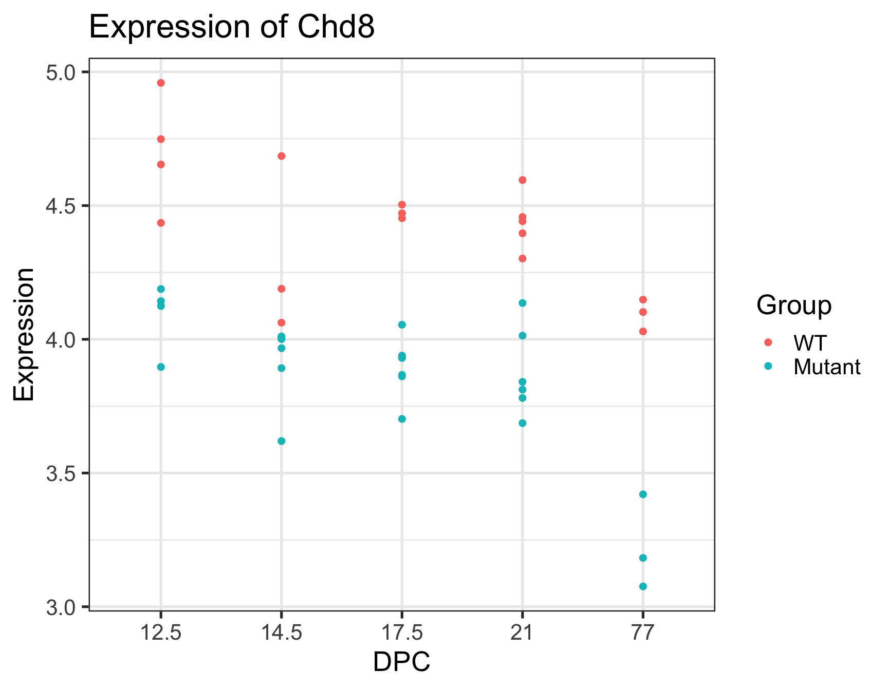
  • Paper reported that CHD8 went down over time, and is lower in the mutant: confirmed!

  • Note that we are not doing any formal “analysis” here nor trying to make this plot beautiful – keeping it very simple for our exploration

Two views of the same data: Which do you prefer?

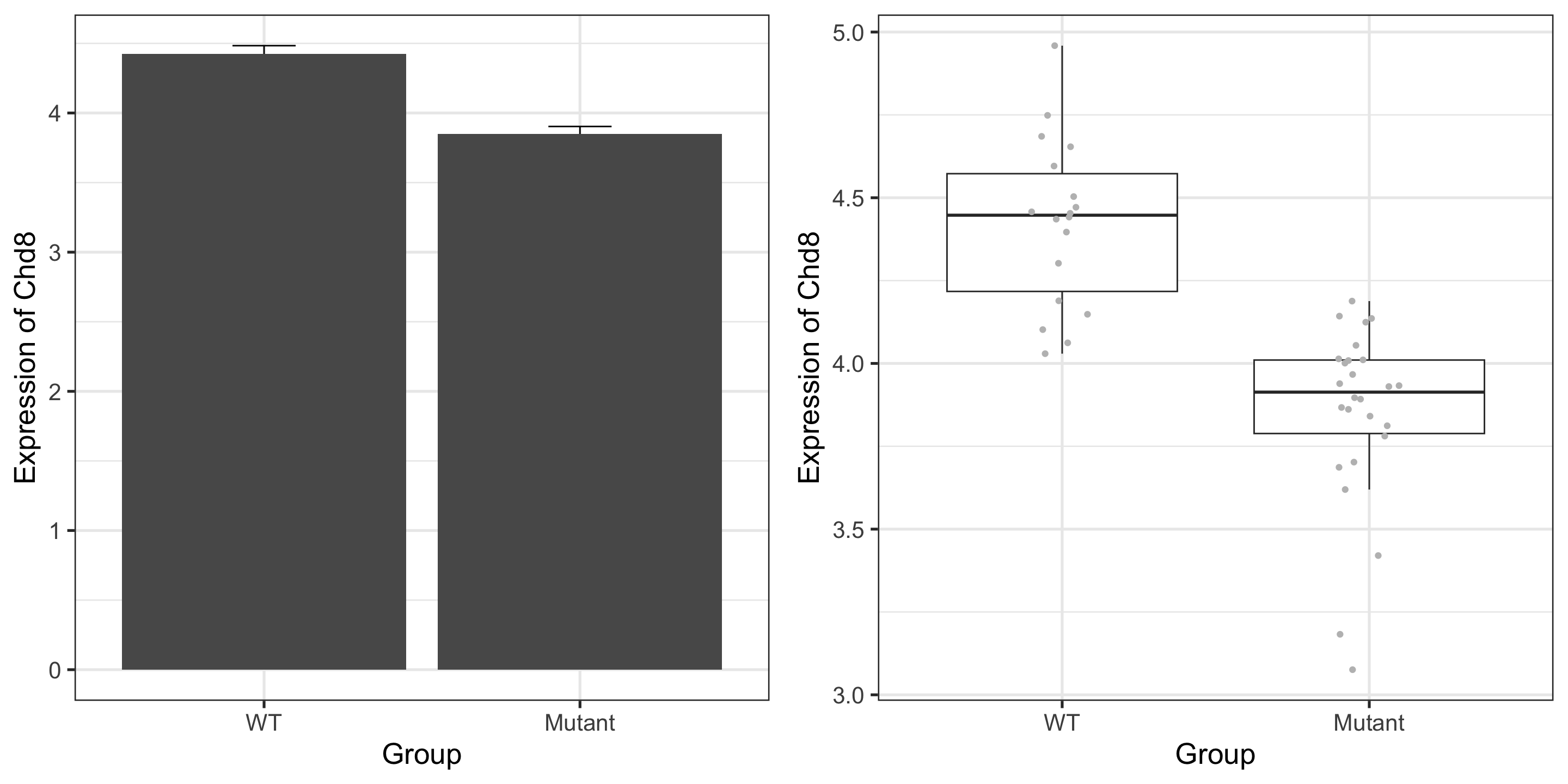
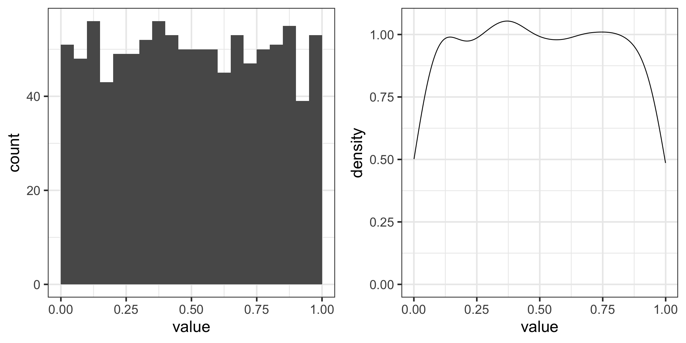
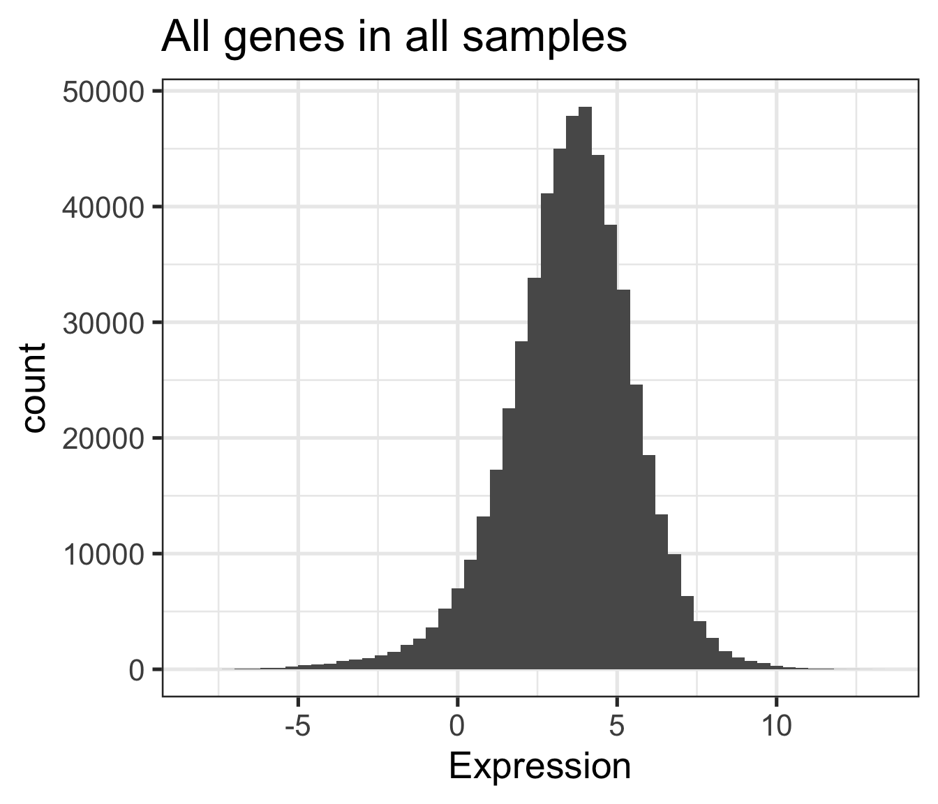
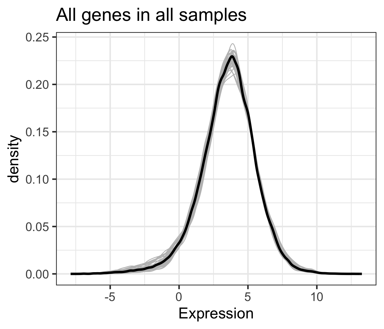
How to best summarize patterns in the data?

Two views of the same data: Let the data speak for itself!

  • What is the sample size?

  • Is the distribution symmetrical, or skewed?

  • Are there any outliers?

Comparing sample distributions: Boxplots

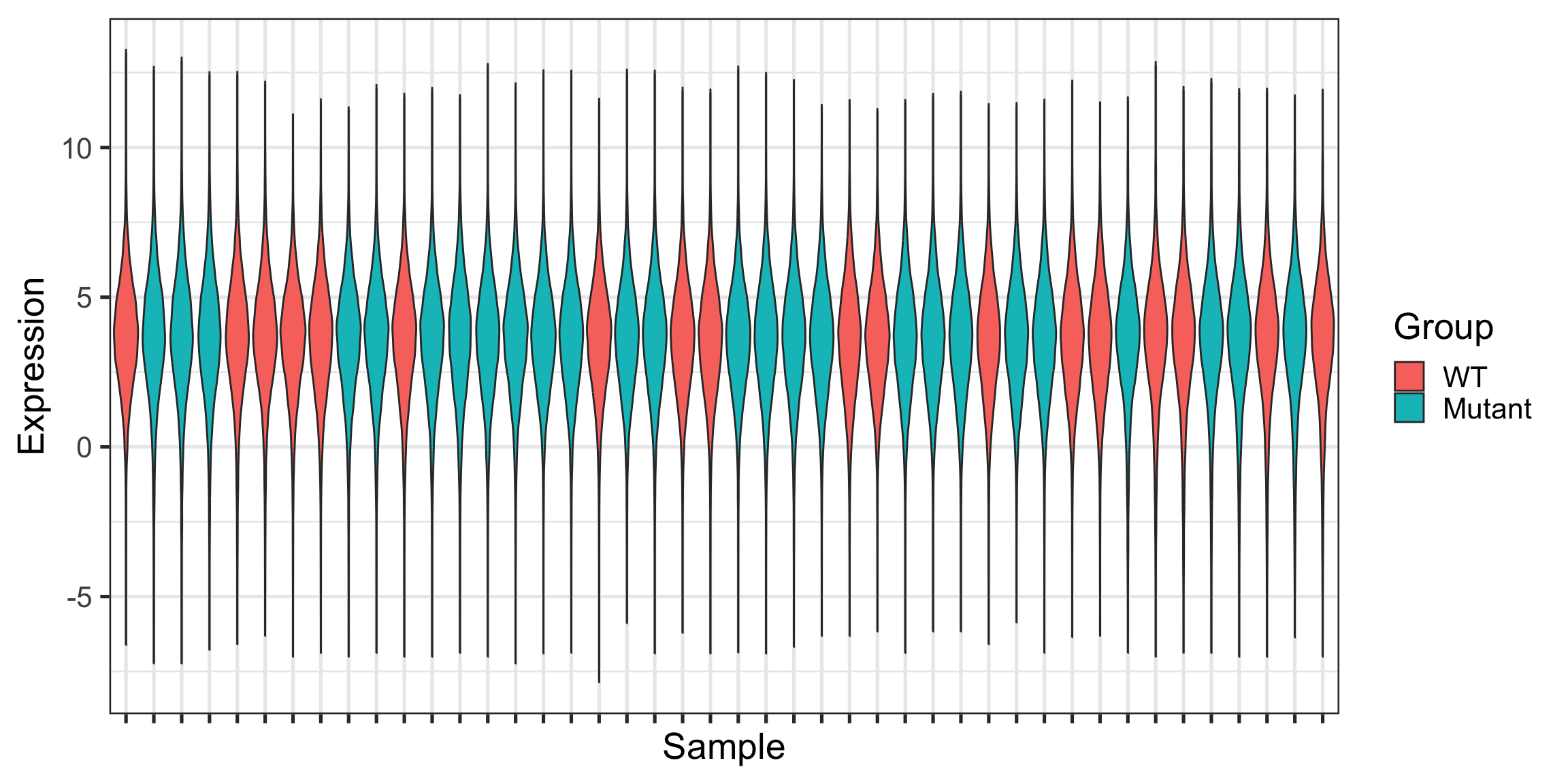
  • Quick and dirty; reasonable tool to summarize large amounts of data

  • Not ideal if the distribution is multimodal

  • Don’t use box plots (alone) when you have small numbers of points; show the points instead!

Comparing distributions: Histograms and Density plots

Don’t use density plots for bounded data

Violin plots

A hybrid of density plots and box plots

Scatter plots

Major problem is ‘over-plotting’ - use transparency or 2D density

Transformations

  • Many real data have very skewed distributions – in this case, most values are <500, but there are a smattering up to 10,000
  • If your plots look like this, try taking the logarithm
  • If have non-positive values (typically 0) add a small constant “pseudocount”

Pairwise (scatter) plots to compare samples

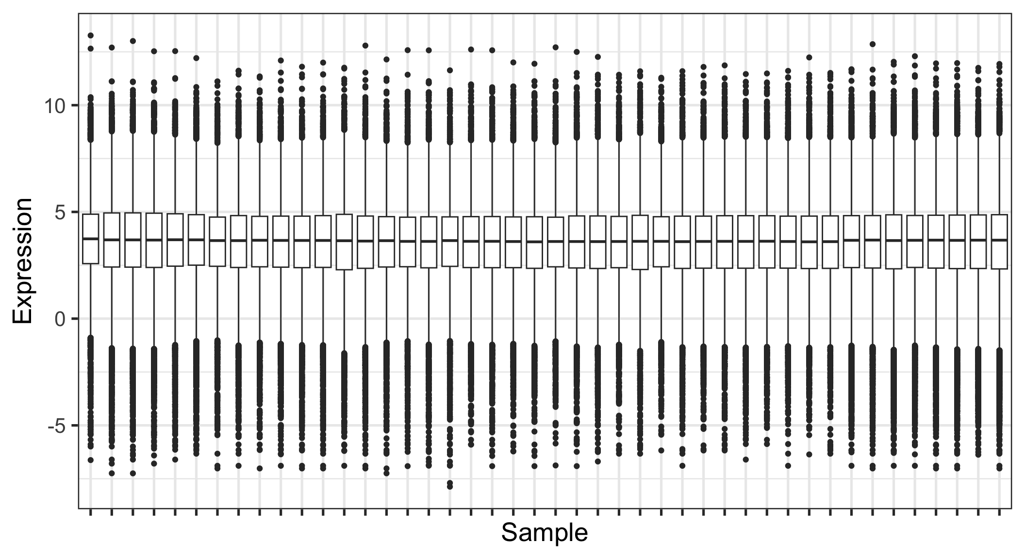
This is nice but unwieldy (or won’t work) for large data sets

Examining the metadata more globally

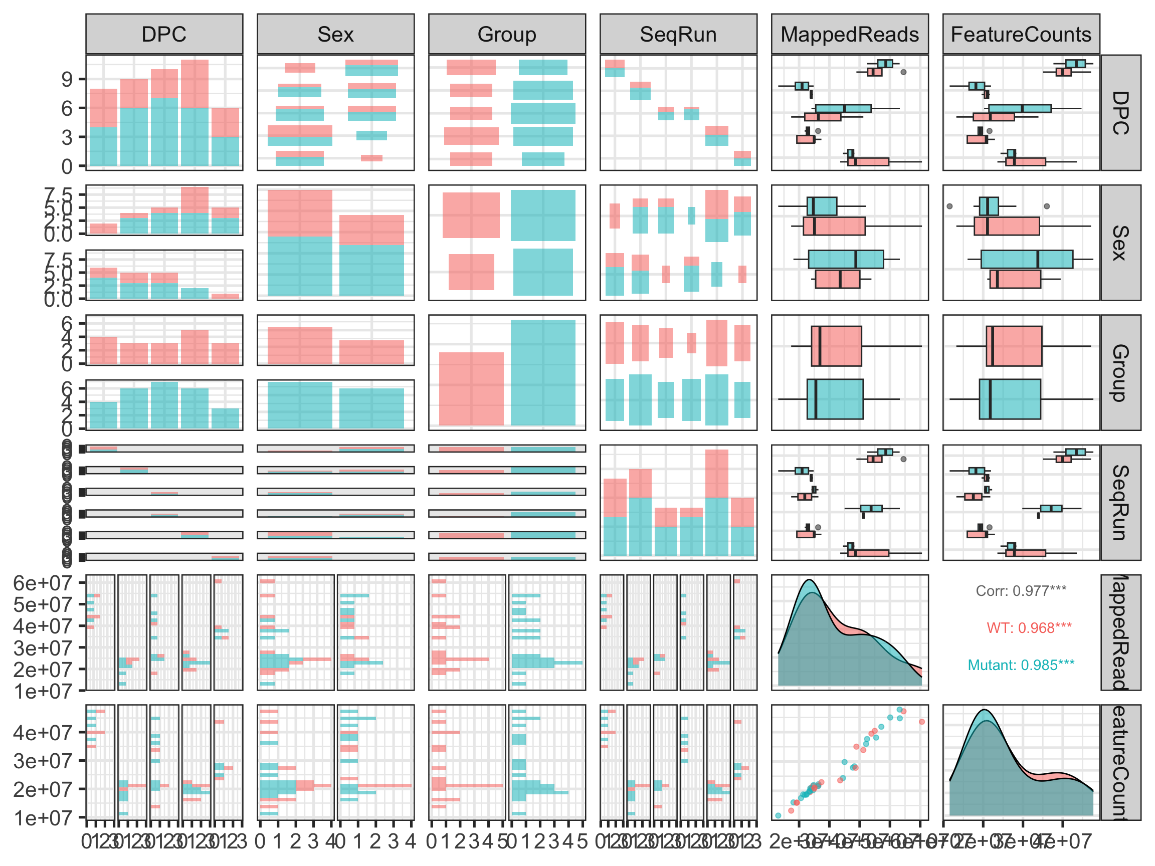
  • Sex is not that well balanced

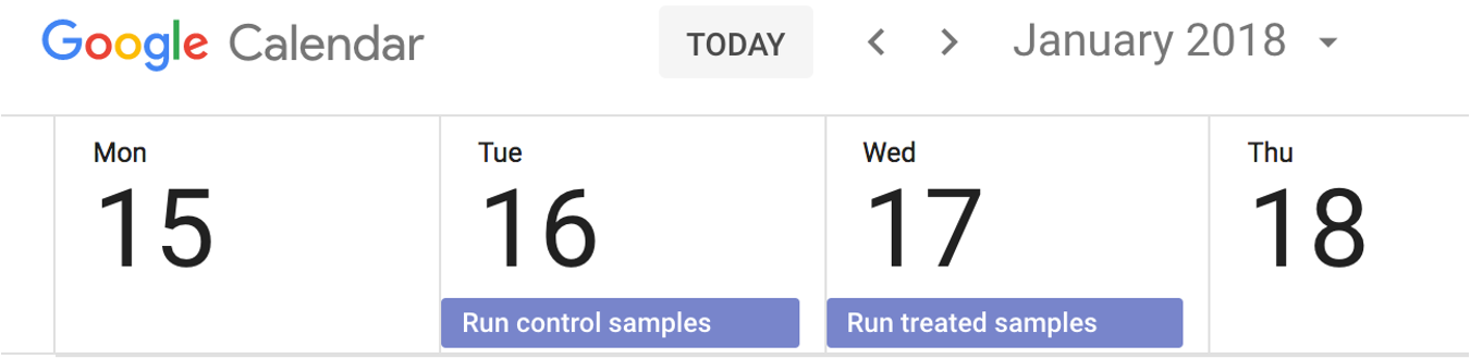
  • There is a batch confound: The stages were run in different batches (except 17.5 was split in two)

  • Mapped reads varies with the batches (SeqRun)

Heatmaps

R options for making heatmaps

  • Desired features
    • Doesn’t complain when handed slightly messy data and has sensible default behaviour

    • Allow easy control of layout such as annotations and scale bar

    • Allow easy control over clustering behaviour (row/column ordering)

  • There are many functions/packages for making heatmaps; here are three
    • base::heatmap - ok for quick and dirty but otherwise very limited

    • pheatmap - Default colour schemes not ideal, otherwise good option (used in STAT 540 seminars)

    • ComplexHeatmaps - most powerful/flexible, but a bit more complex to learn

Heatmap of 50 random rows

Revision 1: Same input data; rows are scaled

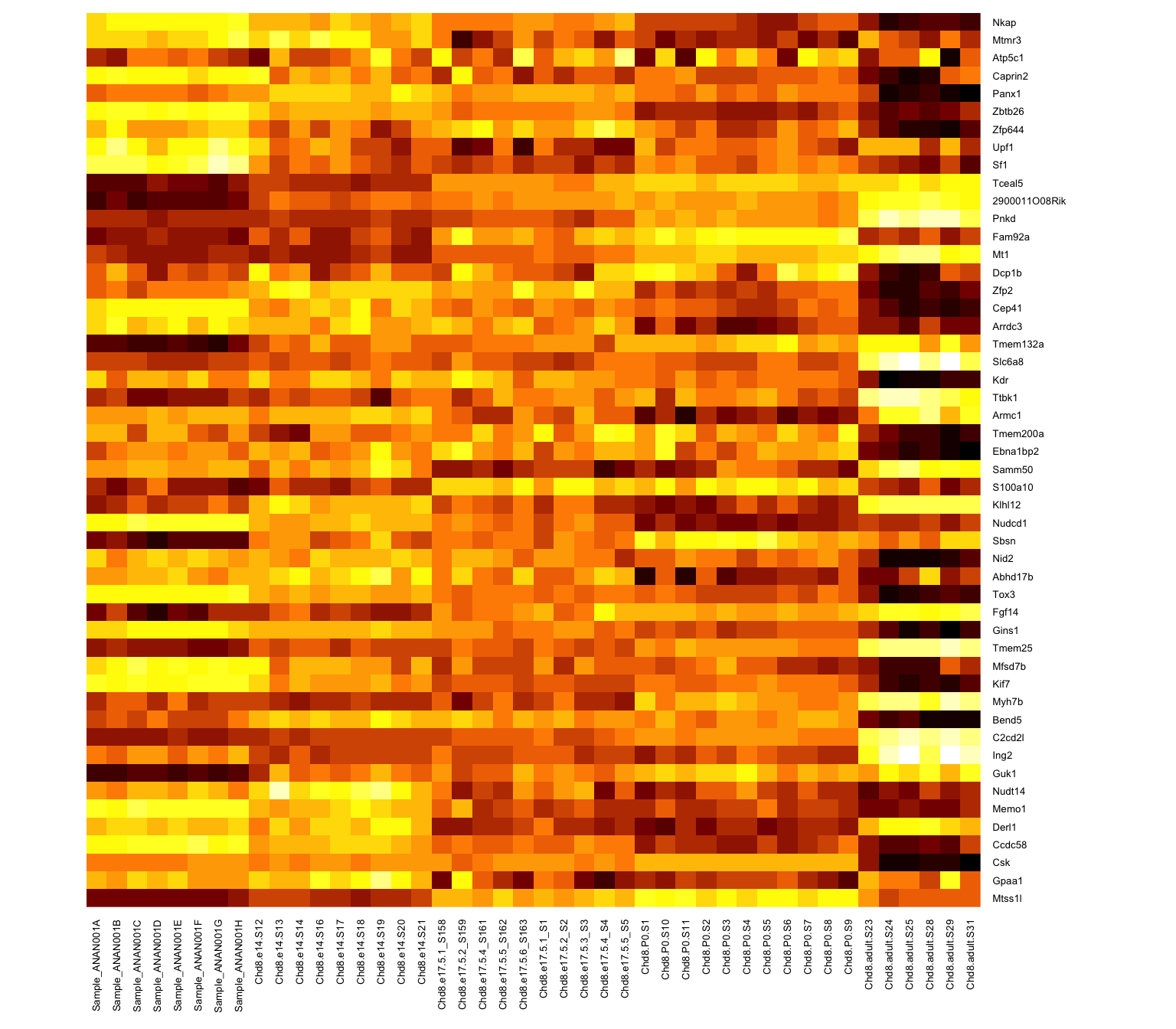
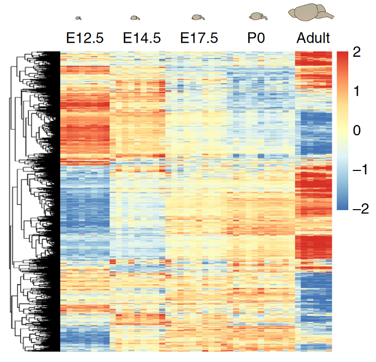
  • Rows are scaled to have mean 0 and variance 1 (z-scores)

  • Subtract the mean; divide by the standard deviation - use scale() on the data rows (some packages will do this by default)

  • It is now easier to compare the rows and see a bit of structure

Revision 2: adjusting contrast

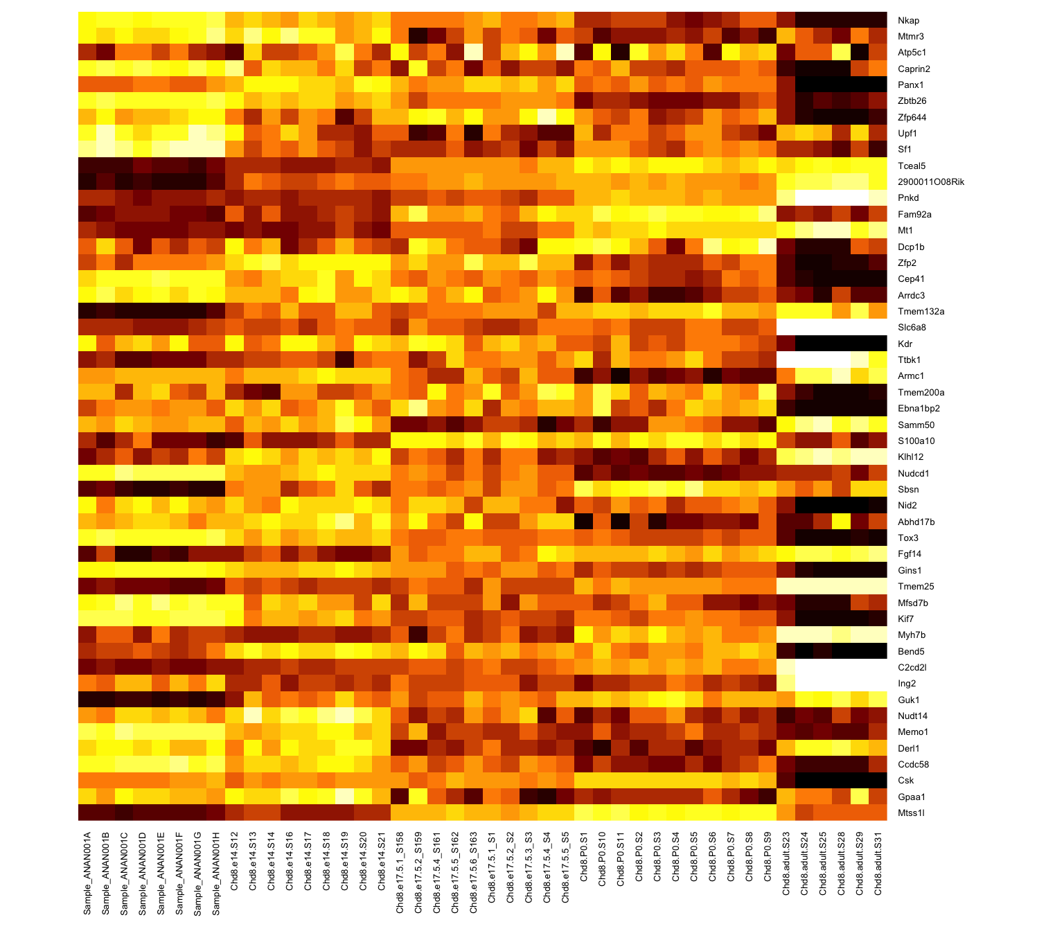
  • Range of values is clipped to (-2,2): aything more than two SDs from the row mean is set to 2

  • Limit values of 2 or 3 SDs are common

Clipping hides outliers but allows us to see variation in the bulk of the data

Plotting too much data

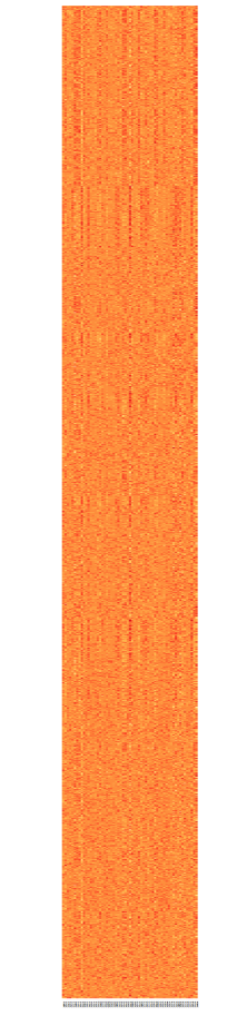
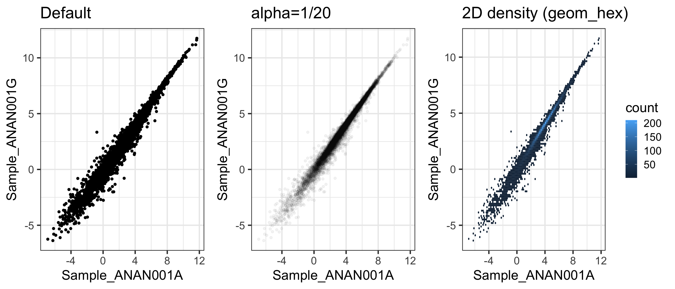
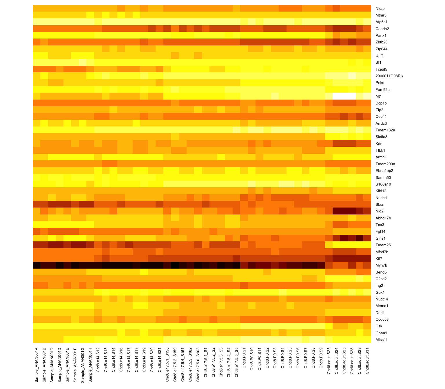
  • An entire data set (>10k rows)

  • If the cells are less than 1 pixel, everything starts to turn to mush and can even be misleading

  • If your heatmap has too many rows to see labels (genes), make sure it is conveying useful information (what are you trying to show?)

Choice of colours

  • Humans can’t really tell the difference between a 8- and 16-colour scale
  • Many R defaults, other common scales (green/red) not colourblind friendly
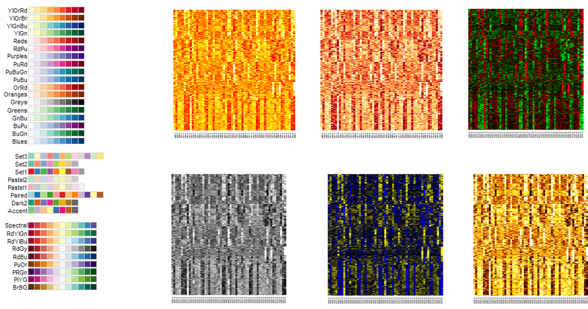
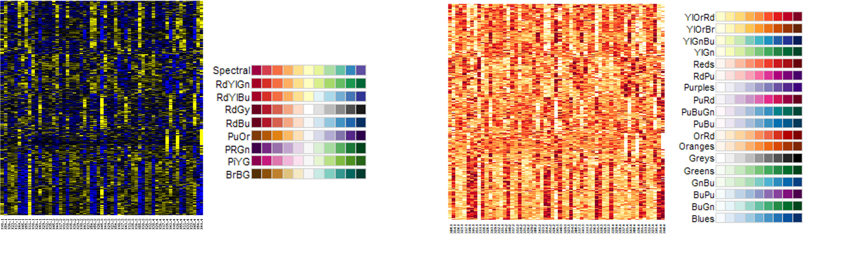
  • RColorBrewer: scales based on work of visualization experts
  • Greyscale: loss of dynamic range, but cheaper to publish!

Divergent vs. sequential maps

Divergent: colours pass through black or white at the midpoint (e.g. mean). Ideal if your original data are naturally “symmetric” around zero (or some other value) - Otherwise it might just be confusing

Sequential: colours go from light to dark. Darker colours mean “higher” by default in RColorBrewer. No defined midpoint.

A confusing heat map (Matlab)

  • Too many different colours to readily interpret relative ordering of values

  • Not recommended to use these types of scales for continuous values

  • Rainbows or scales with many distinct colours are better for factors / categorical variables

Heatmap recommendations

  • Pick an appropriate colour scale

  • Show a scale bar (so don’t use base::heatmap)

  • Either cluster rows / columns, or order by something meaningful (e.g. sample info)

  • Add annotation bars of meaningful covariates

  • If you have missing data points, make sure it is obvious where they are (e.g. different colour)

EDA Summary

Purpose: Evaluate whether data aligns with expectations:

  • Sanity checks
  • Visualization to spot patterns and/or oddities

Four principles of EDA:

  1. Let the data speak for itself - avoid dynamite plots in favor of boxplots, overlayed with points if feasible number

  2. Avoid overplotting - use transparency or 2D density in scatterplots; make sure heatmap cells aren’t too small

  3. Consider transformations (e.g. log) for skewed distributions

  4. Use colour intentionally to convey information

Additional exploratory techniques will be discussed later in the course (e.g. Clustering, PCA)

Experimental design and quality

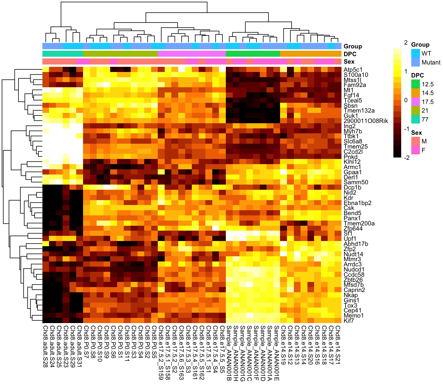
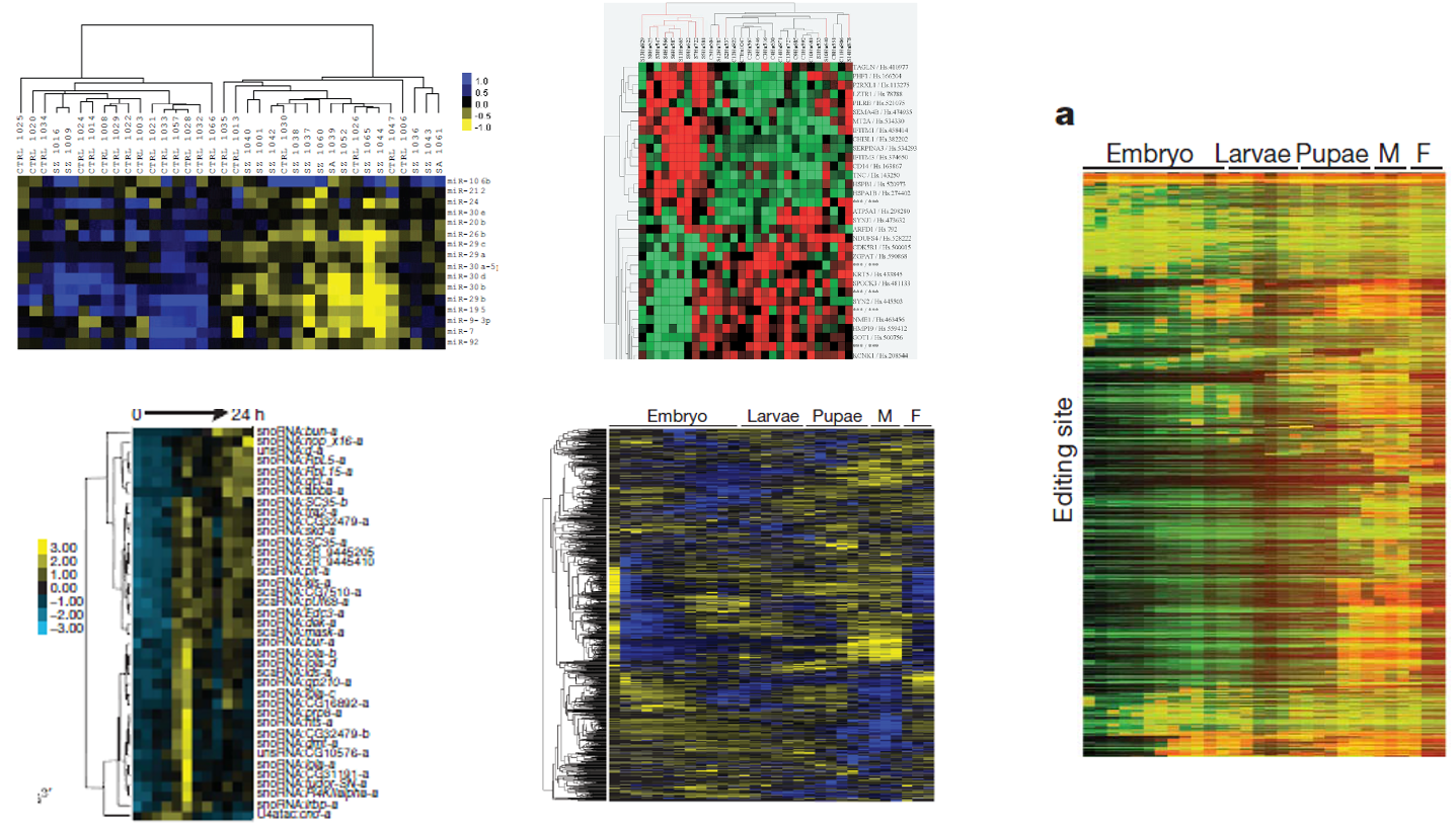
Fig 1, 10.1038/sj.ebd.6400436

Experimental design considerations

  • Will the experiment answer the question?
    • Consider properties of the measurement technology as well as the biology
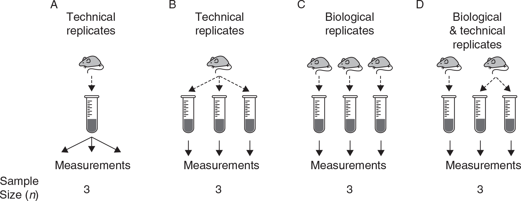
  • How many individuals should I study?
    • For many experiments, this is hard to answer (even though your grant reviewer might demand it (power calculations)!)
    • Often settle for “enough power to find something useful” rather than “find everything”
  • Biological replicates are essential and more important than technical replicates (usually)
    • Doing a study with too few replicates is arguably worse than not doing the study
  • Beware of (and try to control for) unwanted variation
    • “Pooling” samples is not a substitute for replication
    • E.g. if your question is “do people respond to a drug”, the unit of analysis must be Person, not Group of people

Data quality considerations

General types of issues:

  • High technical variability

  • Outliers

  • Batch artifacts (or other systematic trends)

Effects on the data:

  • Some will yield false positives (confounds, “false signals”)

  • Others will yield false negatives (by decreasing signal-to-noise)

Filtering your data

  • Here I mean “Removing part of the data from a sample” and doing that to all samples

  • In many studies, especially gene expression, it is common to remove genes that have no or very low signal (“not expressed”)

  • Deciding what to remove is often not straighforward, but make a principled decision and stick with it (see next slide)

Filters must be “unsupervised”

  • Filtering strategy should treat all samples the same

  • Filtering strategy should be decided up front

Batch effects

“Batch effects are sub-groups of measurements that have qualitatively different behaviour across conditions and are unrelated to the biological or scientific variables in a study”

Leek et al. 2010 Nature Rev. Genetics 11:733

  • Magnitude of batch effects vary

  • Consider correcting for them if possible - batch artifact detection and correction will be covered in more detail in a later lecture

Avoiding batch artifacts

  • Don’t samples run in batches - Confounding (can be hard to avoid)
  • Balance or randomize design with respect to batches
  • Avoid (or at least record) obvious potential sources of artifacts, such as a new tube of a reagent, or a different person doing the bench work
  • Run some technical replicates across your batches
table(se$DPC, se$SeqRun)
      
        A  B  C  D  E  H
  12.5  8  0  0  0  0  0
  14.5  0  9  0  0  0  0
  17.5  0  0  5  5  0  0
  21    0  0  0  0 11  0
  77    0  0  0  0  0  6

Outliers

Hard to define

  • “A sample that deviates significantly from the rest of the samples in its class”

  • “An observation differing widely from the rest of the data.”

  • “A data point notably further out from the central value than the others. Outliers invite explanation as observational errors, or intrusions from another set, or something of that sort.”

  • “… a value that lies 1.5 IQR beyond the upper or lower quartile”

Features (e.g. genes) are not usually called “outliers” in the sense of “should remove from the data”

Identifying outlier samples

  • Relative vs. absolute quality is important

  • We might consider a sample an outlier if (relative to others):

    • It has “very low” signals
    • “High” background
    • “Low” correlation with most (or all) other samples from the same group
    • There may be technology-specific factors
  • If a sample is questionable, we might ask: Is there anything suspect in the experimental process? (e.g. “Sample dropped on floor”)
    – this will help justify decisions to remove a sample beyond arbitrary criteria like “>1.5 IQR”

A basic but effective outlier detection method

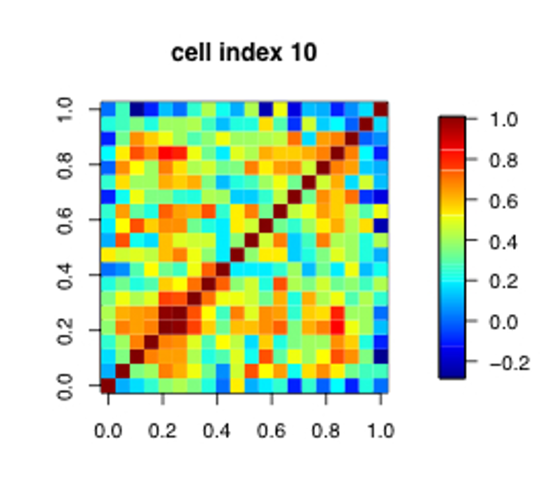
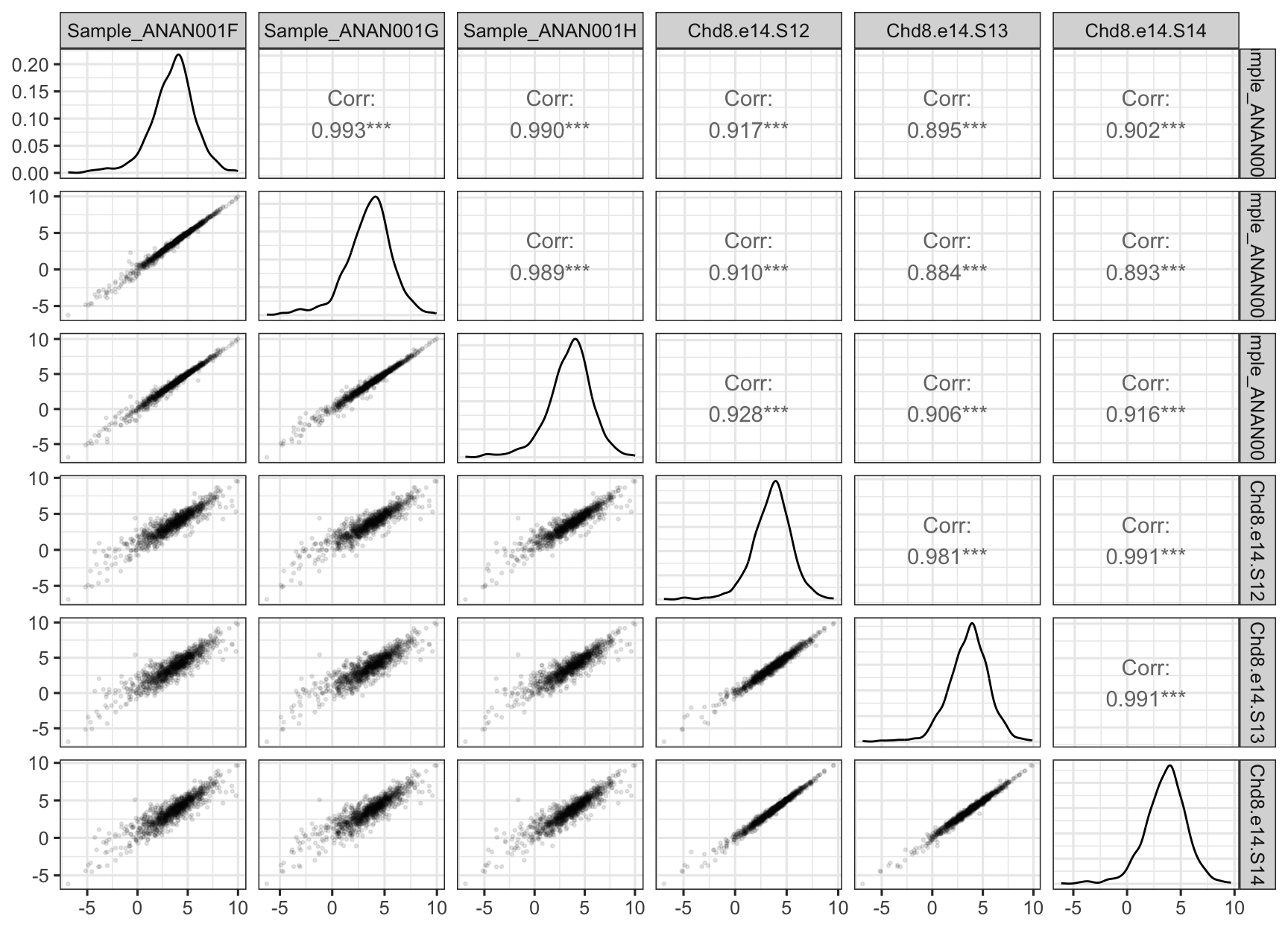
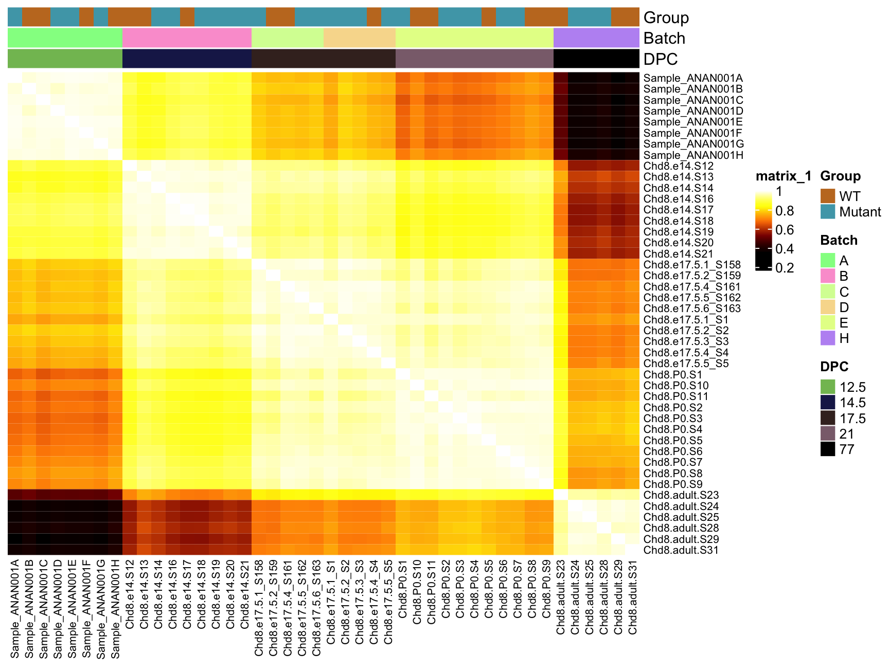
A heatmap of the sample-sample correlation matrix (generally a useful diagnostic plot)

Expect correlations to be tighter within experimental groups than across groups

  • There are no firm guidelines for evaluating this … but you could apply a rule like “out of >1.5 IQR”

  • In practice, outliers are often pretty obvious