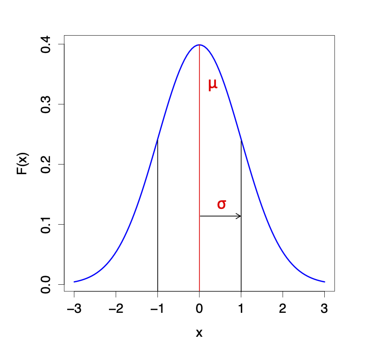
Let’s say we collected a sample from a population we assume to be normal
We estimate the mean \(\large \hat{\mu}=\bar{x}\)
How good is the estimate?
Sampling distribution
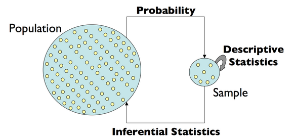
Statistic: any quantity computed from values in a sample
Any function (or statistic) of a sample (data) is a random variable
Thus, any statistic (because it is random) has its own probability distribution function \(\rightarrow\) specifically, we call this the sampling distribution
Example: the sampling distribution of the mean
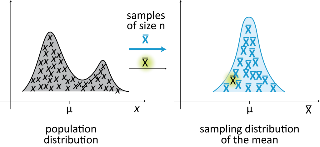
Sampling distribution of the mean
The sample mean \(\large \bar{x}\) is a RV, so it has a probability or sampling distribution
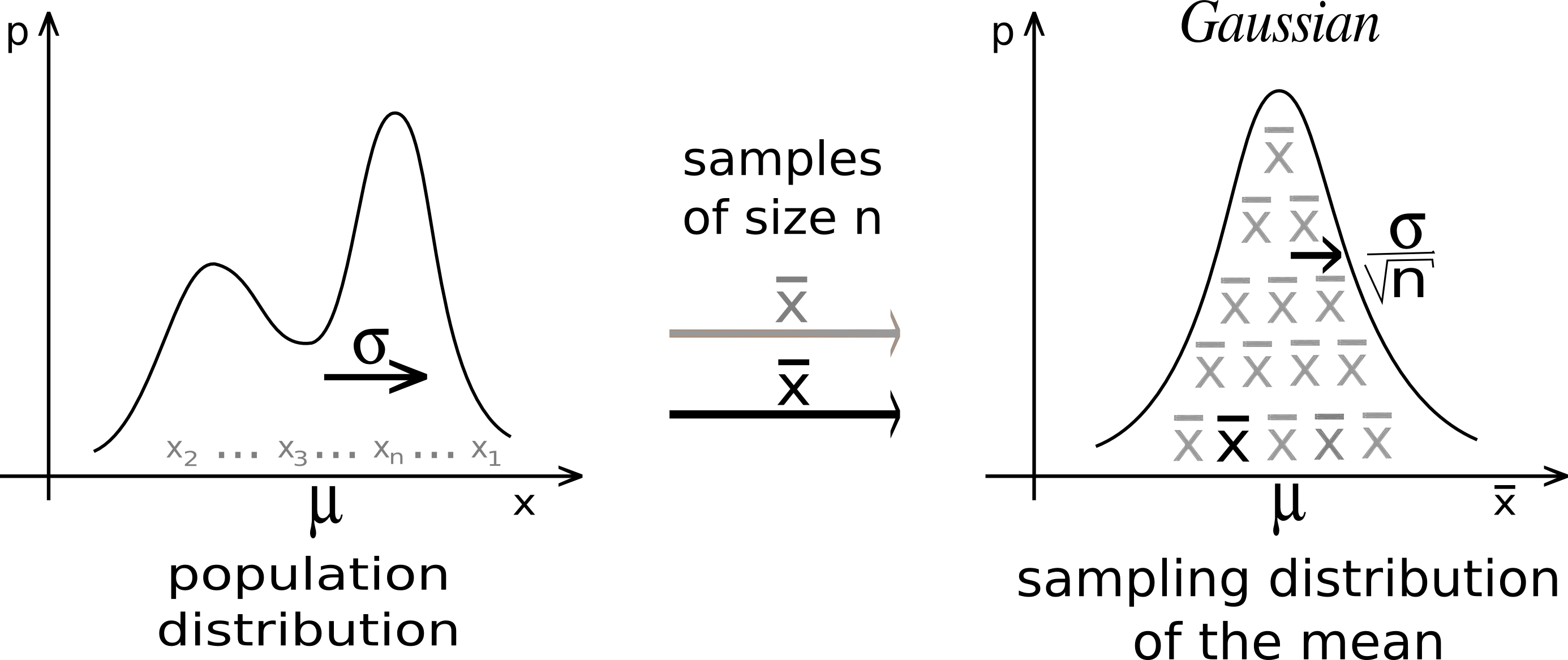
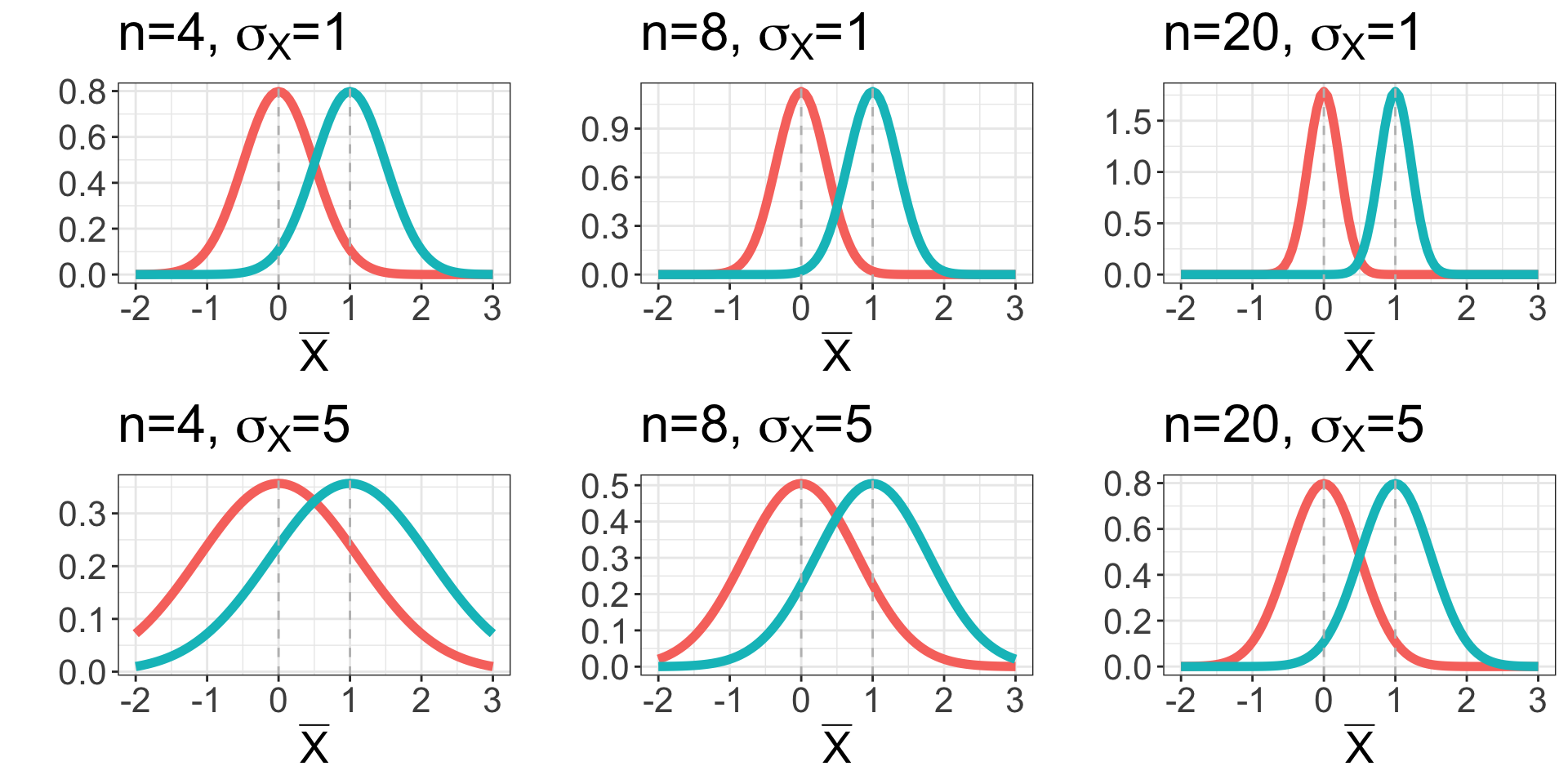
By the Central Limit Theorem (CLT), we know that the sampling distribution of the mean (of \(n\) observations) is Normal with mean \(\mu_{\bar{X}} = \mu\) and standard deviation \(\sigma_{\bar{X}} = \frac{\sigma}{\sqrt{n}}\)
The standard deviation is not the same as the standard error
Standard error describes variability across multiple samples in a population
Standard deviation describes variability within a single sample
The sampling distribution of the mean of \(n\) observations (by CLT): \[\bar{X} \sim N(\mu, \frac{\sigma^2}{n})\]
The standard error of the mean is \(\frac{\sigma}{\sqrt{n}}\)
The standard deviation of \(X\) is \(\sigma\)
Estimation of parameters of the sampling distribution of the mean
Just as we estimated \(\mu\) and \(\sigma\) for our sample of \(n\) observations from a normally distributed population before, we can also estimate \(\mu_{\bar{X}}\) and \(\sigma_{\bar{X}}\):
The standard error (SE) of the mean reflects uncertainty about our estimate of the population mean\(\large\hat{\mu}\)
For the distributional assumptions to hold, the CLT assumes a ‘large enough’ sample:
Rule of thumb: when the sample size is ~30 or more, the normal distribution is a good approximation for the sampling distribution of the mean
for smaller samples, the SE \(\large\frac{s}{\sqrt{n}}\) is an underestimate
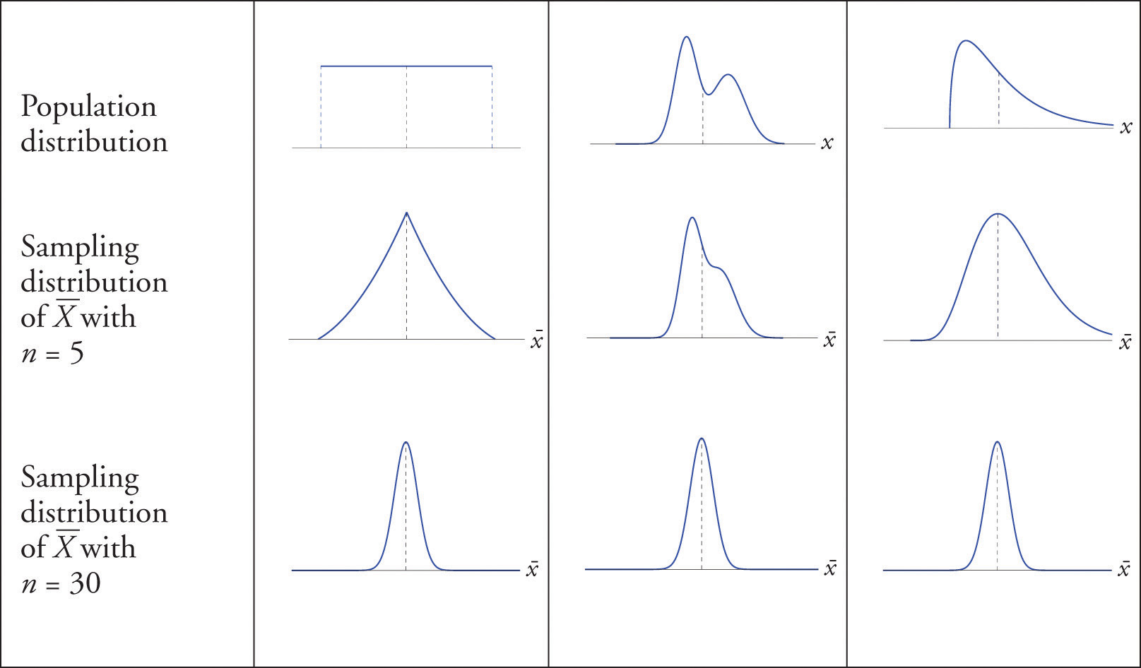
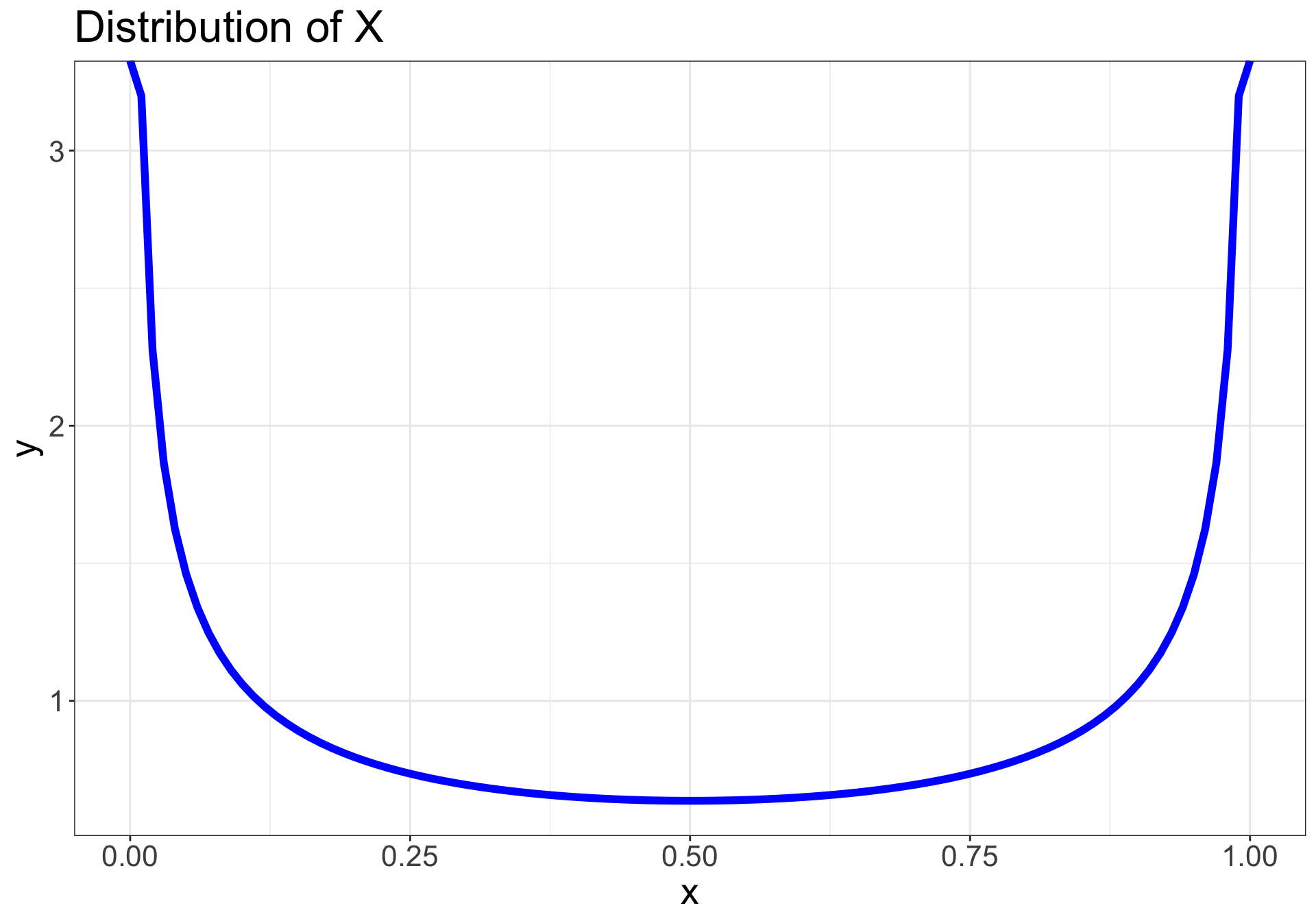
CLT applies to any population…
…regardless of distribution
Let \(\normalsize X_1, X_2, ..., X_n\) be a random sample from a population with a non-normal distribution
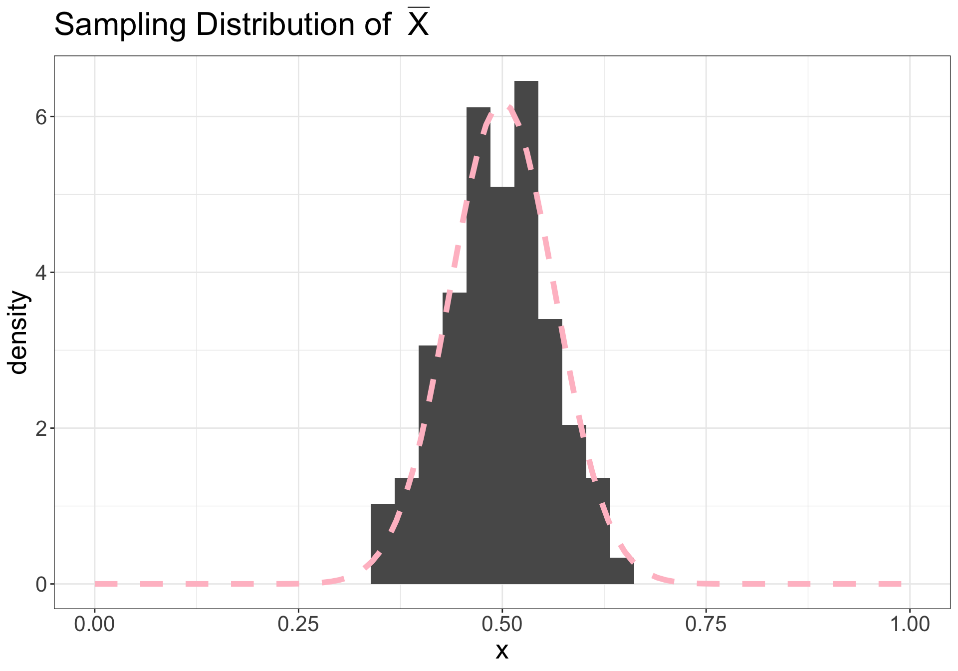
If the sample size \(\normalsize n\) is sufficiently large, then the sampling distribution of the mean will be approximately normal: \(\normalsize \bar{X} \sim N(\mu, \frac{\sigma^2}{n})\)
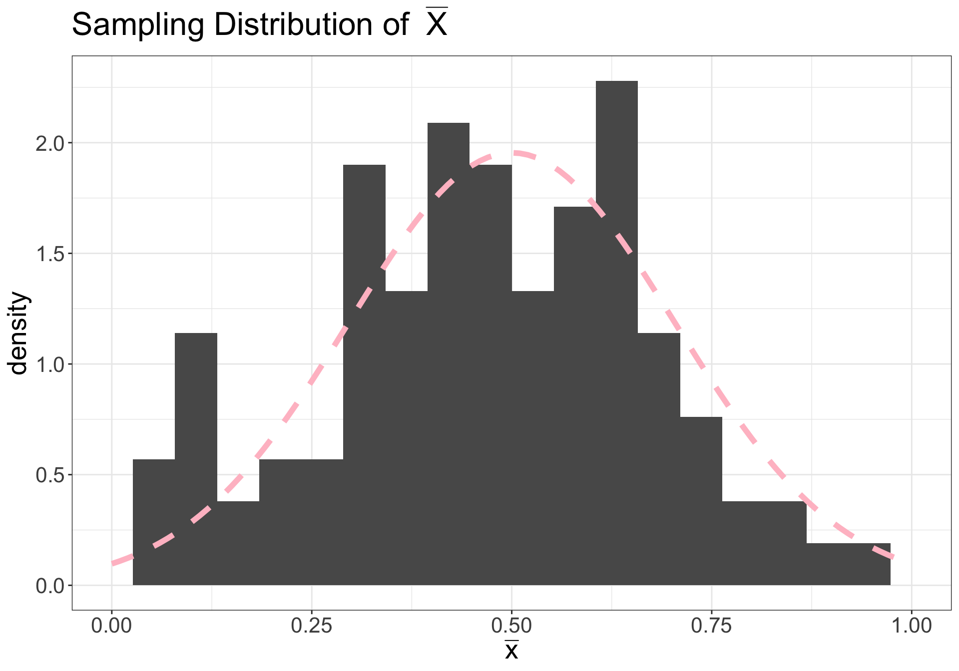
On right: dashed pink line is \(N(\mu, \sigma^2/n)\)
Illustration (n = 10)
On right: dashed pink line is \(N(\mu, \sigma^2/n)\)
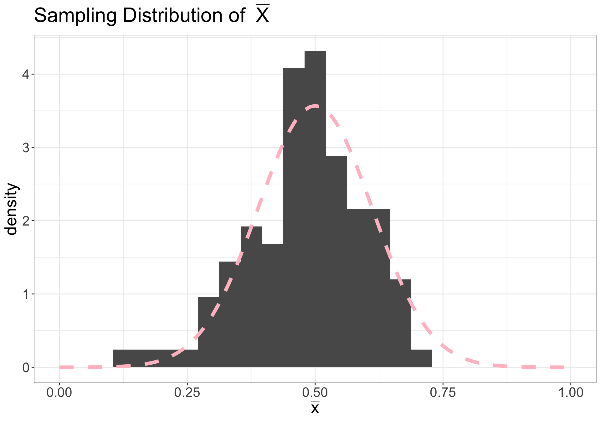
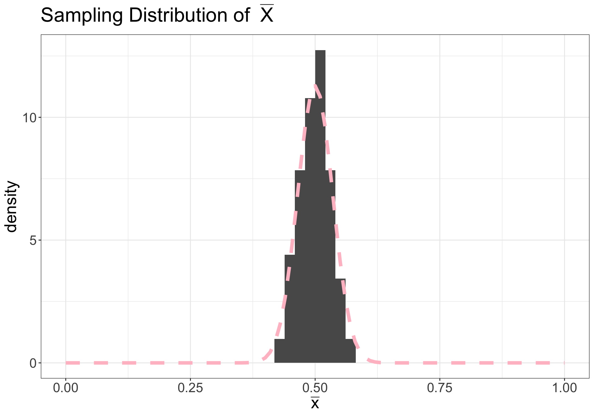
Illustration (n = 30)
On right: dashed pink line is \(N(\mu, \sigma^2/n)\)
Illustration (n = 100)
On right: dashed pink line is \(N(\mu, \sigma^2/n)\)
Hypothesis Testing
Hypothesis: A testable (falsifiable) idea for explaining a phenomenon
Statistical hypothesis: A hypothesis that is testable on the basis of observing a process that is modeled via a set of random variables
Hypothesis Testing: A formal procedure for determining whether to accept or reject a statistical hypothesis
Requires comparing two hypotheses:
\(H_0\): null hypothesis
\(H_A\) or \(H_1\): alternative hypothesis
Hypothesis Testing: Motivating Example
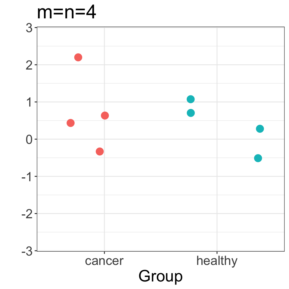
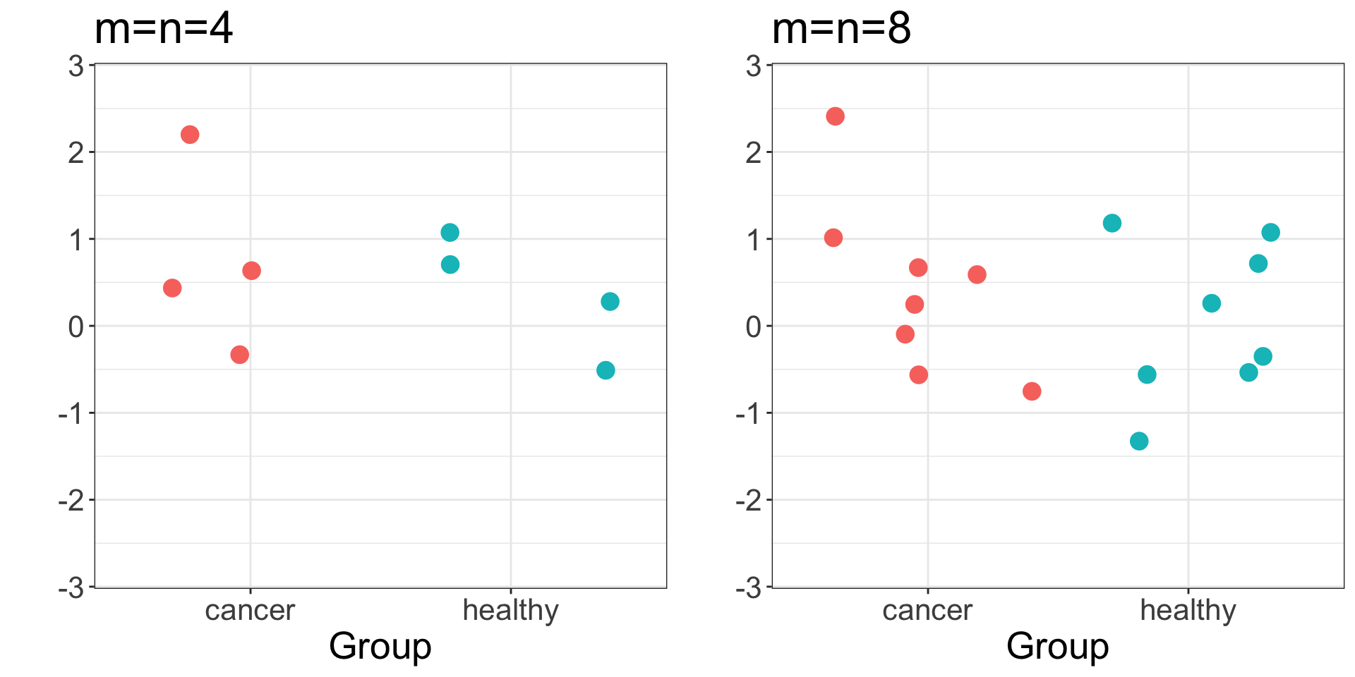
The expression level of gene \(\normalsize g\) is measured in \(\normalsize n\) patients with disease (e.g. cancer), and \(\normalsize m\) healthy (control) individuals:
Is gene \(\normalsize g\) differentially expressed in cancer vs healthy samples?
\(\normalsize H_0: \mu_Z = \mu_Y\)
\(\normalsize H_A: \mu_Z \neq \mu_Y\)
In this setting, hypothesis testing allows us to determine whether observed differences between groups in our data are significant
Steps in Hypothesis Testing
Formulate your hypothesis as a statistical hypothesis
Define a test statistic \(t\) (RV) that corresponds to the question. You need to know the expected distribution of the test statistic under the null
Compute the p-value associated with the observed test statistic under the null distribution \(\normalsize p(t | H_0)\)
Motivating example (cancer vs healthy gene expression)
Motivating example (cancer vs healthy gene expression)
Motivating example (cancer vs healthy gene expression)
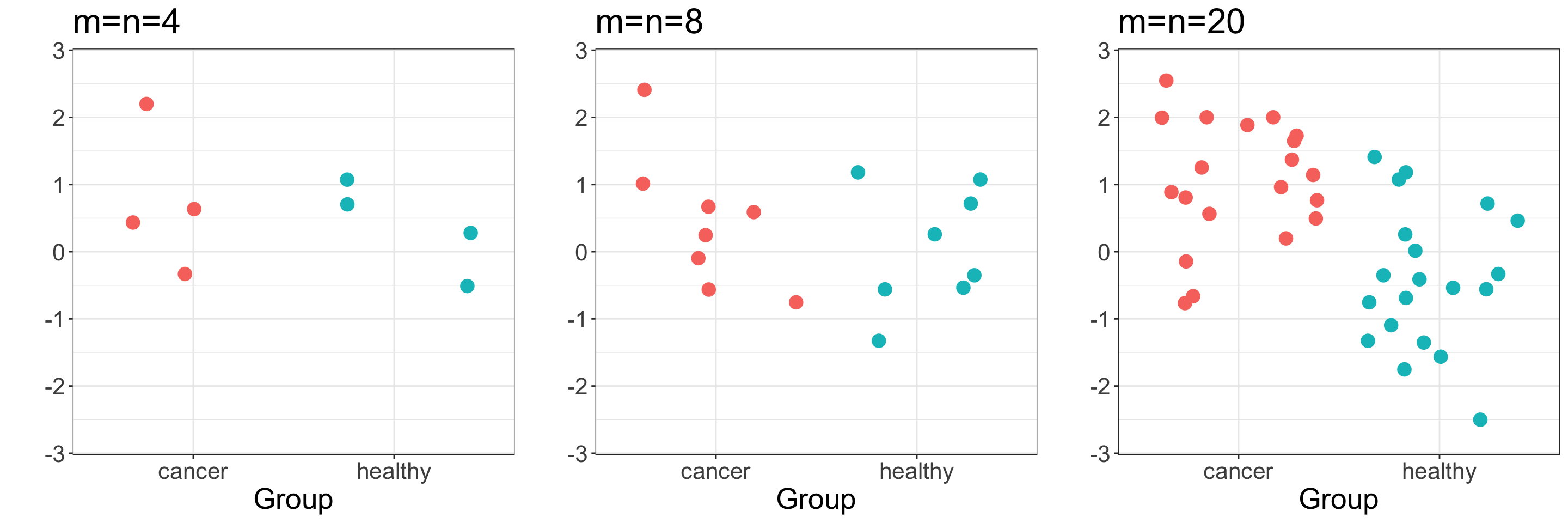
Is there a significant difference between the two means?
Samples drawn from independent Normal distributions with equal variance and \(\mu_Z-\mu_Y=1\)
Is there a significant difference between the two means?
Which panel looks most significant?
Which looks least significant?
Is there a significant difference between the two means?
Mean difference needs to be put into context of the __________________ and __________________. Recall the formula for the sampling distribution of the mean:
2 sample t-statistic
2-sample t-statistic: measures difference in means, adjusted for spread/standard deviation:
\[\normalsize t=\frac{\bar{z}-\bar{y}}{SE_{\bar{z}-\bar{y}}}\] e.g. for \(z_1, z_2, ..., z_n\) expression measurements in healthy samples and \(y_1, y_2, ..., y_m\) cancer samples
From the theory, we know the distribution of our test statistic, if we are willing to make some assumptions
2 sample t-test
If we assume:
\(\bar{Z}\) and \(\bar{Y}\) are normally distributed
\(Z\) and \(Y\) have equal variance
Then the standard error estimate for the difference in means is: