Linear models with multiple factors

Keegan Korthauer

February 1, 2024

Project next steps - written proposal

Details here
Expand upon your proposal lightning talk, incorporating feedback
Include a plan for how team will work together
- Aim for a fair balance
- It is acceptable to modularize your overall workflow, assigning each team member some of the components (e.g. one group member performs planned analysis A, another group member perfroms planned analysis B, etc)
- It is not acceptable for one group member to take on sole responsibility of the tasks of a certain type (e.g. one group member doing all of the analysis, or one group member defining the research question and hypotheses, etc)

Last class…

How to compare means of different groups (2 or more) using a linear regression model
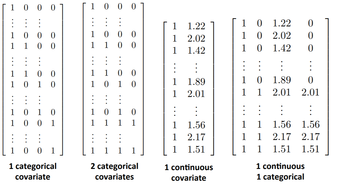
- indicator variables to model the levels of a qualitative explanatory variable
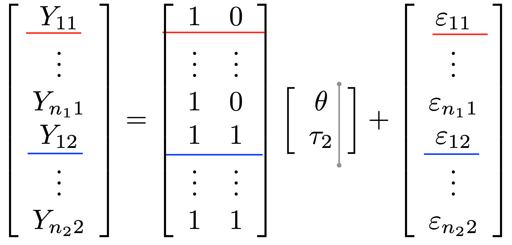
Write a linear model using matrix notation
- understand which matrix is built by R
Distinguish between single and joint hypotheses
- \(t\)-tests vs \(F\)-tests

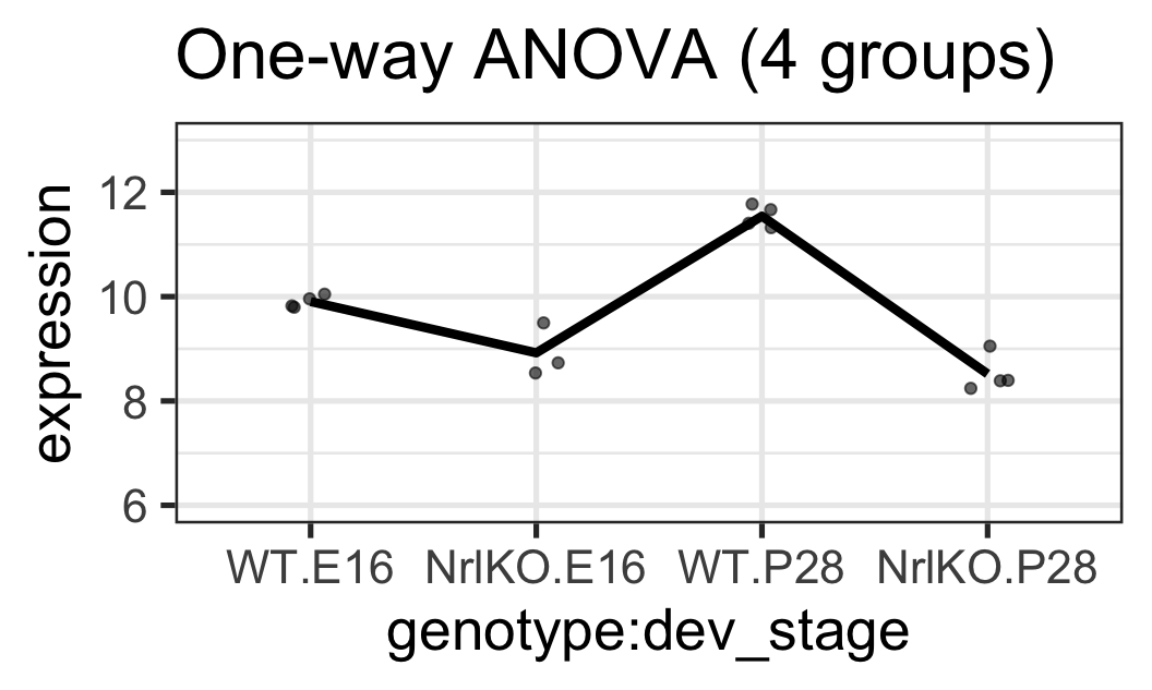
Comparing more than two groups

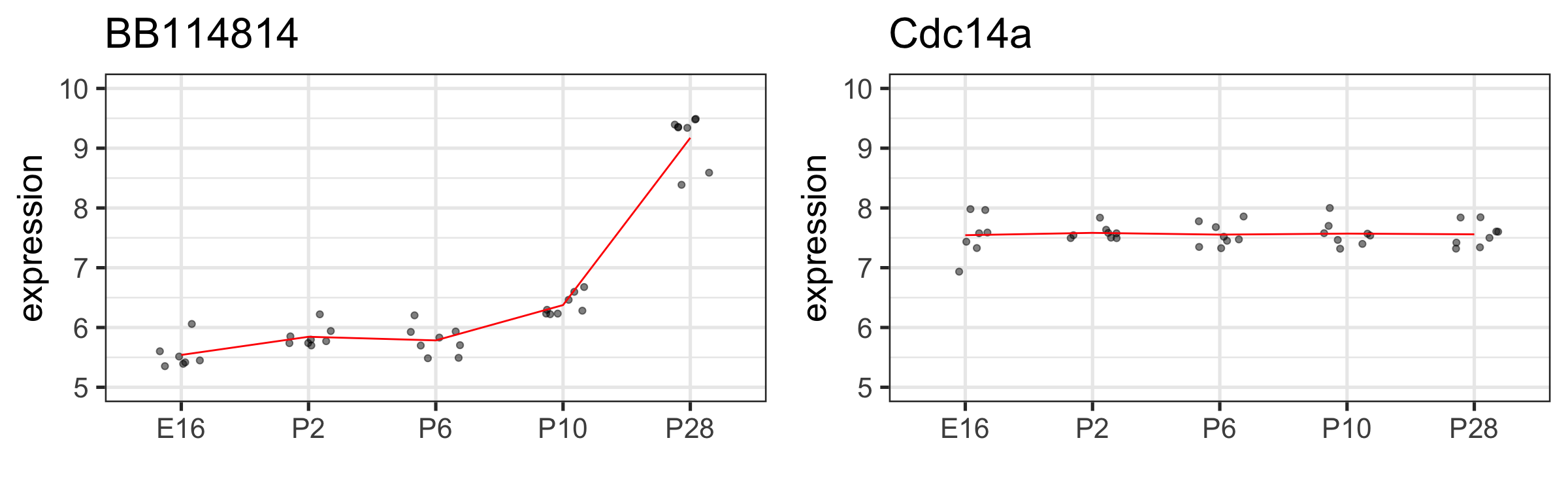
Biological question: do gene expression levels differ by developmental stage?
Statistical question: are gene expression generated by a single common distribution across all developmental stages? Or do the distributions differ by timepoint?

Code

bb1plot <- twoGenes %>% filter(gene == "BB114814") %>%
  ggplot(aes(x = dev_stage, y = expression)) + 
             geom_jitter(width = 0.2, alpha = 0.5) +
             labs(title = "BB114814") +
             theme(legend.position = "none") +
             ylim(5, 10) +
             xlab("") +
             stat_summary(aes(group=1), fun=mean, geom="line", colour="red")

cdcplot <- twoGenes %>% filter(gene == "Cdc14a") %>%
  ggplot(aes(x = dev_stage, y = expression)) + 
             geom_jitter(width = 0.2, alpha = 0.5) +
             labs(title = "Cdc14a") +
             theme(legend.position = "none") +
             ylim(5, 10) +
             xlab("") +
             stat_summary(aes(group=1), fun=mean, geom="line", colour="red")
grid.arrange(bb1plot, cdcplot, nrow = 1)

Quick review: from \(t\)-test to linear regression

2-sample t-test

\[ Y \sim F; \ E[Y]= \mu_Y ; \ Z \sim G; \ E[Z]= \mu_Z \] \[ H_0: \mu_Y = \mu_Z\]

↓

How? Why?

↓

Linear regression

\[ Y = X\alpha + \epsilon; \text{ }\hspace{1em} H_0: \alpha_j = 0\]

How: Cell means model using indicator variables

\[ Y \sim F; \ E[Y]= \mu_Y ; \ Z \sim G; \ E[Z]= \mu_Z \]

\[Y_{ij}= \mu_1 x_{ij1} + \mu_2 x_{ij2} + \varepsilon_{ij}; \ i=1, \dots, n; \ j={1,2}\] \[x_{ij1}=\bigg\{\begin{array}{l} 1\text{ if } j=1\\ 0 \text{ otherwise}\\ \end{array}, \hspace{1em} x_{ij2}=\bigg\{\begin{array}{l} 1\text{ if } j=2\\ 0 \text{ otherwise}\\ \end{array}\]

\[\begin{array}{l} E[Y_{i1}] &= \mu_1 \\ E[Y_{i2}] &= \mu_2 \end{array}\]

How: Reference-treatment parameterization using indicator variables

\[ Y \sim F; \ E[Y]= \mu_Y ; \ Z \sim G; \ E[Z]= \mu_Z \]

\[Y_{ij}=\theta+ \tau_2 x_{ij2} + \varepsilon_{ij}; \ i=1, \dots, n; \ j={1,2}\] \[x_{ij2}=\bigg\{\begin{array}{l} 1\text{ if } j=2\\ 0 \text{ otherwise}\\ \end{array}\]

\[\begin{array}{l} E[Y_{i1}] &= \theta=\mu_1 \\ E[Y_{i2}] &= \theta + \tau_2=\mu_1\ + (\mu_2 - \mu_1) = \mu_2 \end{array}\]

How: Using matrix notation

2 group comparison:

\(Y_{ij}=\theta+ \tau_2 x_{ij2} + \varepsilon_{ij}\) → \(\bf{Y} = \bf{X\alpha+\epsilon}\)

\(x_{ij2}\) is the second column of \(X\) (design matrix)
Tip: examine design matrix in R with model.matrix()

\[\color{red}{Y_{11} = 1*\theta + 0*\tau_2 + \epsilon_{11} =\theta + \epsilon_{11}}\]

\[\color{blue}{Y_{12} = 1*\theta + 1*\tau_2 + \epsilon_{12} = \theta + \tau_2 + \epsilon_{12}}\]

Recall

For comparisons involving more than 2 groups (ANOVA), we add indicator variables (columns of \(X\))

Why: Flexible framework

\(\bf{Y} = \bf{X\alpha+\epsilon}\) gives us a very flexible framework

These (and many more) can be accommodated by the design matrix (X)!

Parameterizations

Different ways of writing the \(\bf{X\alpha}=\) [design matrix][parameter vector] pair correspond to different parameterizations of the model

\[\bf{Y} = \bf{X\alpha} + \varepsilon\]

Understanding these concepts makes it easier:

to interpret and compare fitted models
to fit models such that comparisons you care most about are directly addressed in the output

Example: compare means between groups

By default, lm estimates group mean differences (with respect to a reference group):

filter(twoGenes, gene == "BB114814") %>%
  lm(expression ~ dev_stage, data = .) %>%
  tidy()

# A tibble: 5 × 5
  term         estimate std.error statistic  p.value
  <chr>           <dbl>     <dbl>     <dbl>    <dbl>
1 (Intercept)     5.54      0.102     54.2  1.31e-34
2 dev_stageP2     0.304     0.140      2.17 3.69e- 2
3 dev_stageP6     0.243     0.140      1.74 9.11e- 2
4 dev_stageP10    0.834     0.140      5.96 9.62e- 7
5 dev_stageP28    3.63      0.140     26.0  5.30e-24

We can tell R to use the cell-means parameterization

Write the formula as Y ~ 0 + x in the lm call to remove the intercept \((\theta)\) parameter and fit cell means parameters instead

filter(twoGenes, gene == "BB114814") %>%
  lm(expression ~ 0 + dev_stage, data = .) %>%
  tidy()

# A tibble: 5 × 5
  term         estimate std.error statistic  p.value
  <chr>           <dbl>     <dbl>     <dbl>    <dbl>
1 dev_stageE16     5.54    0.102       54.2 1.31e-34
2 dev_stageP2      5.84    0.0956      61.2 2.30e-36
3 dev_stageP6      5.78    0.0956      60.5 3.27e-36
4 dev_stageP10     6.38    0.0956      66.7 1.23e-37
5 dev_stageP28     9.17    0.0956      96.0 5.56e-43

What null hypotheses does the t-test column now represent?

Converting between parameterizations

filter(twoGenes, gene == "BB114814") %>%
  lm(expression ~ 0 + dev_stage, data = .) %>%
  tidy()

# A tibble: 5 × 5
  term         estimate std.error statistic  p.value
  <chr>           <dbl>     <dbl>     <dbl>    <dbl>
1 dev_stageE16     5.54    0.102       54.2 1.31e-34
2 dev_stageP2      5.84    0.0956      61.2 2.30e-36
3 dev_stageP6      5.78    0.0956      60.5 3.27e-36
4 dev_stageP10     6.38    0.0956      66.7 1.23e-37
5 dev_stageP28     9.17    0.0956      96.0 5.56e-43

filter(twoGenes, gene == "BB114814") %>%
  lm(expression ~ dev_stage, data = .) %>%
  tidy()

# A tibble: 5 × 5
  term         estimate std.error statistic  p.value
  <chr>           <dbl>     <dbl>     <dbl>    <dbl>
1 (Intercept)     5.54      0.102     54.2  1.31e-34
2 dev_stageP2     0.304     0.140      2.17 3.69e- 2
3 dev_stageP6     0.243     0.140      1.74 9.11e- 2
4 dev_stageP10    0.834     0.140      5.96 9.62e- 7
5 dev_stageP28    3.63      0.140     26.0  5.30e-24

Learning objectives for today

Model more than one factor with multiple levels
- build models with multiple categorical variables and their interaction
Distinguish between simple and main effects
- lm vs anova tests
Test main effects using nested models
- \(t\)-tests vs \(F\)-tests

What if you have 2 categorical variables?

For example: genotype and dev_stage (for simplicity, let’s consider only E16 and P28)

ANOVA is usually used to study models with one or more categorical variables (factors)
Can we combine 2 levels in each of 2 factors into 4 groups (treat as one-way ANOVA)?

What if you have 2 categorical variables?

For example: genotype and dev_stage (for simplicity, let’s consider only E16 and P28)

ANOVA is usually used to study models with one or more categorical variables (factors)
Can we combine 2 levels in each of 2 factors into 4 groups (treat as one-way ANOVA)?
- no way to separate effects of each factor, or their interaction

Two-way ANOVA (or a linear model with interaction)

Which group means are we comparing in a model with 2 factors?

\[\mu_1=E[Y_{(WT,E16)}]\] \[\mu_2=E[Y_{(NrlKO,E16)}]\] \[\mu_3=E[Y_{(WT,P28)}]\] \[\mu_4=E[Y_{(NrlKO,P28)}]\]

Reference-treatment effect parameterization

By default, lm assumes a reference-treatment effect parameterization
Mathematically, we just need more indicator variables, see companion notes for more details

twoFactFit <- lm(expression ~ genotype * dev_stage, oneGene)
tidy(twoFactFit)

# A tibble: 4 × 5
  term                       estimate std.error statistic  p.value
  <chr>                         <dbl>     <dbl>     <dbl>    <dbl>
1 (Intercept)                   9.91      0.157     62.9  2.02e-15
2 genotypeNrlKO                -0.984     0.240     -4.09 1.78e- 3
3 dev_stageP28                  1.64      0.223      7.35 1.44e- 5
4 genotypeNrlKO:dev_stageP28   -2.04      0.328     -6.23 6.47e- 5

Cell-means and treatment effects in the two-way model

Why do we need more indicator variables?

table(oneGene$dev_stage, oneGene$genotype)

     
      WT NrlKO
  E16  4     3
  P28  4     4

(means.2Fact <- oneGene %>%
   group_by(dev_stage, genotype) %>% 
   summarize(cellMeans = mean(expression)) %>% 
   ungroup() %>%
   mutate(txEffects = cellMeans - cellMeans[1],
          lmEst = tidy(twoFactFit)$estimate))

# A tibble: 4 × 5
  dev_stage genotype cellMeans txEffects  lmEst
  <fct>     <fct>        <dbl>     <dbl>  <dbl>
1 E16       WT            9.91     0      9.91 
2 E16       NrlKO         8.92    -0.984 -0.984
3 P28       WT           11.5      1.64   1.64 
4 P28       NrlKO         8.52    -1.39  -2.04

What is the reference group here?

Reference group: WT & E16

As before, comparisons are relative to a reference but in this case there is a reference level in each factor: WT and E16

The reference: WT & E16

Mean of reference group: \(\theta=E[Y_{WT,E16}]\)

lm estimate: \(\hat{\theta}\) is the sample mean of the group

tidy(twoFactFit)

# A tibble: 4 × 5
  term                       estimate std.error statistic  p.value
  <chr>                         <dbl>     <dbl>     <dbl>    <dbl>
1 (Intercept)                   9.91      0.157     62.9  2.02e-15
2 genotypeNrlKO                -0.984     0.240     -4.09 1.78e- 3
3 dev_stageP28                  1.64      0.223      7.35 1.44e- 5
4 genotypeNrlKO:dev_stageP28   -2.04      0.328     -6.23 6.47e- 5

means.2Fact

# A tibble: 4 × 5
  dev_stage genotype cellMeans txEffects  lmEst
  <fct>     <fct>        <dbl>     <dbl>  <dbl>
1 E16       WT            9.91     0      9.91 
2 E16       NrlKO         8.92    -0.984 -0.984
3 P28       WT           11.5      1.64   1.64 
4 P28       NrlKO         8.52    -1.39  -2.04

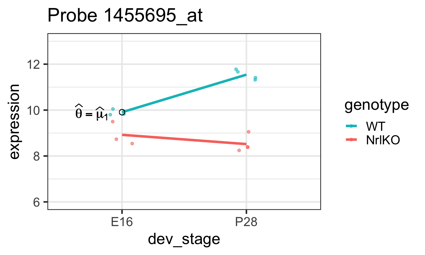
In general, one is not interested in: \(H_0: \theta=0\)

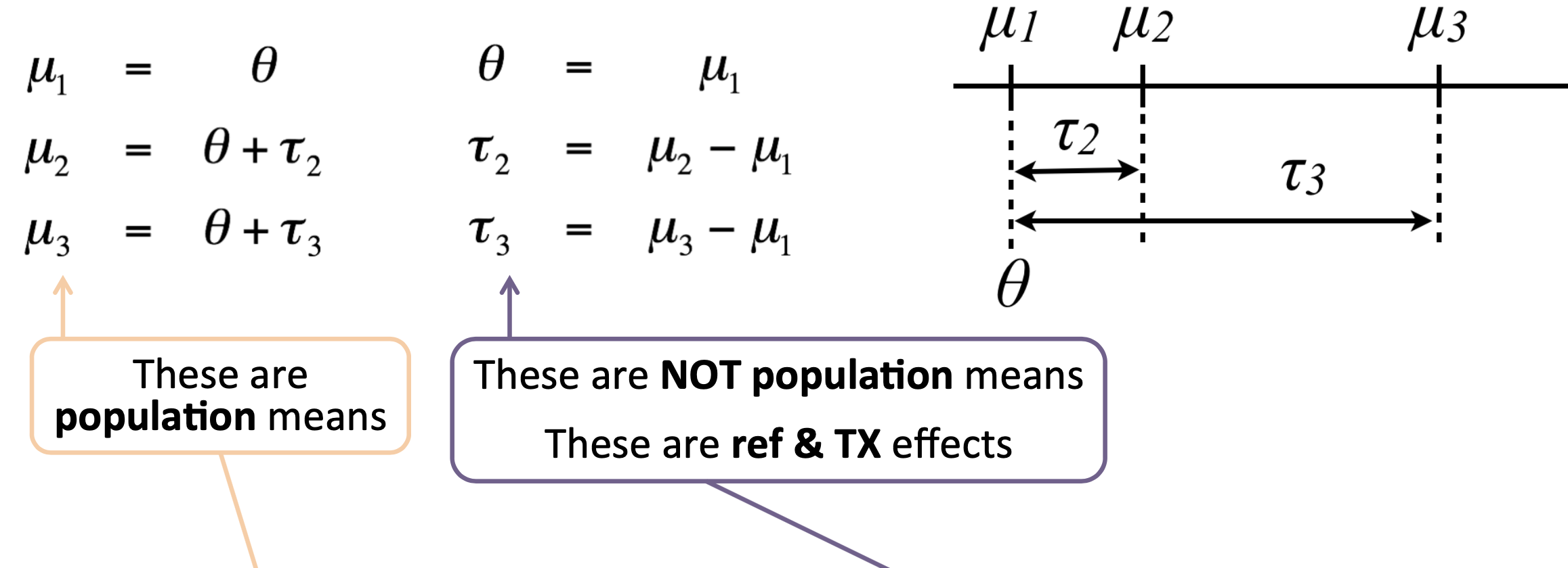
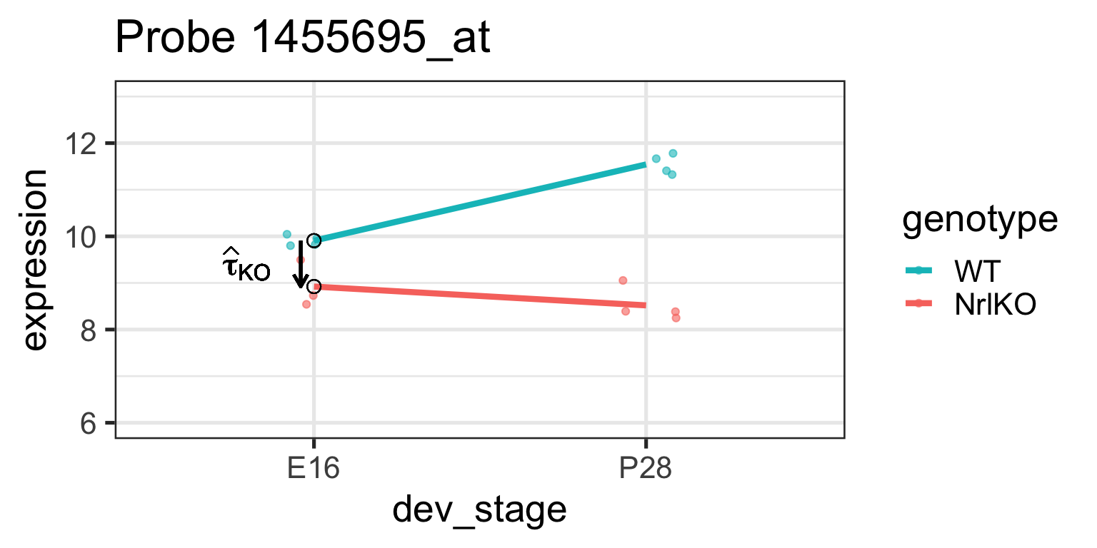
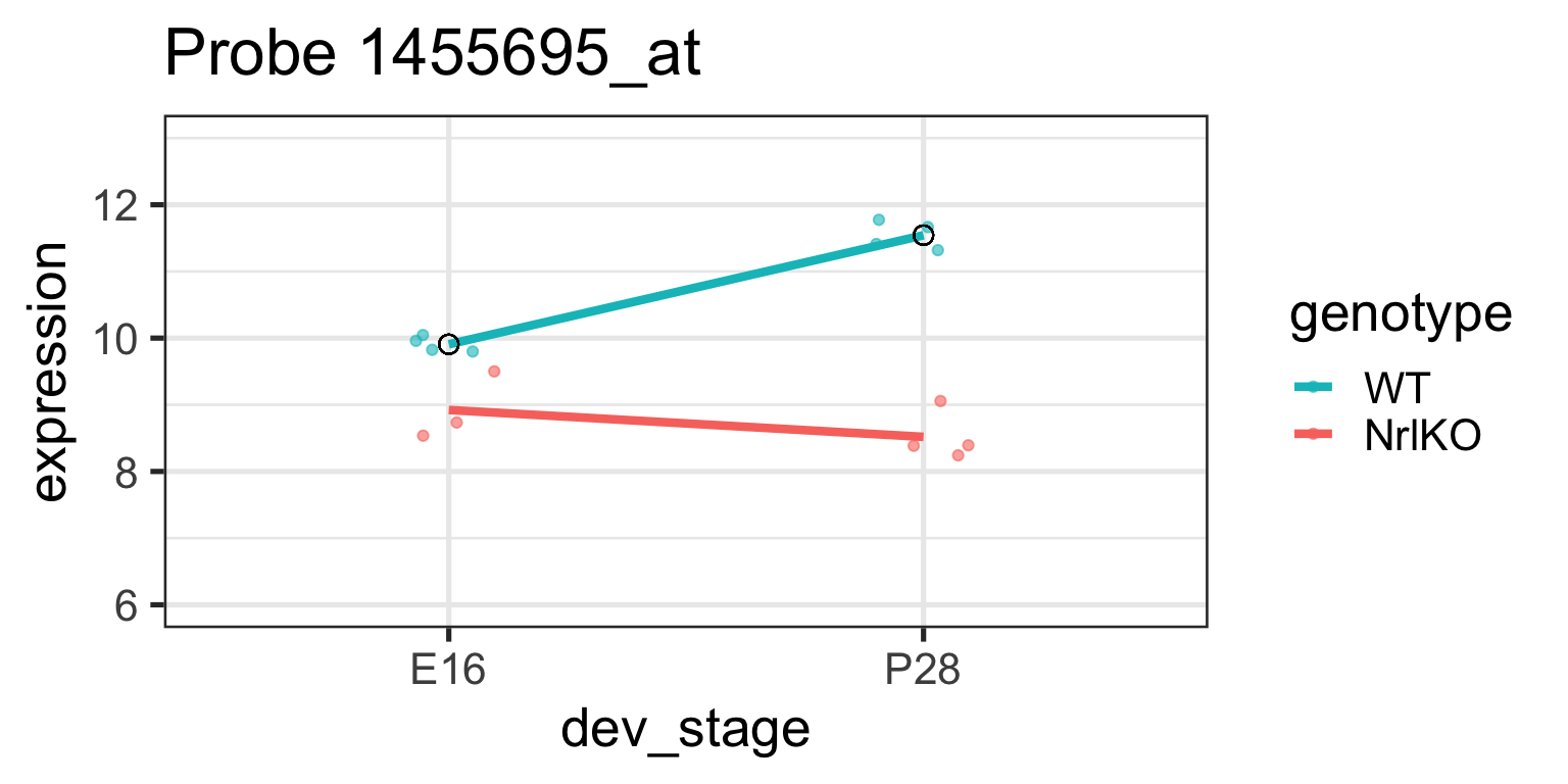
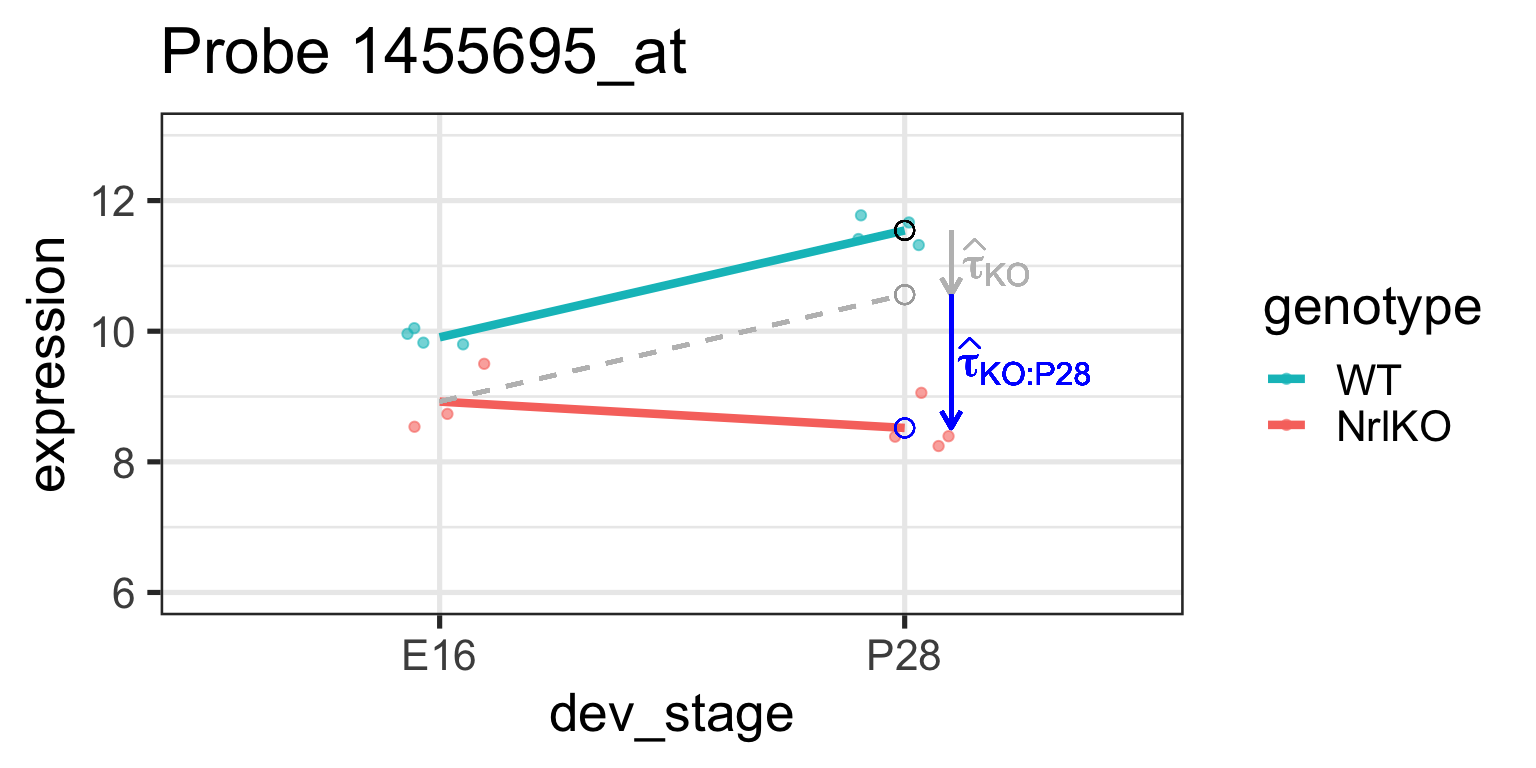
Simple genotype effect: WT vs NrlKO at E16

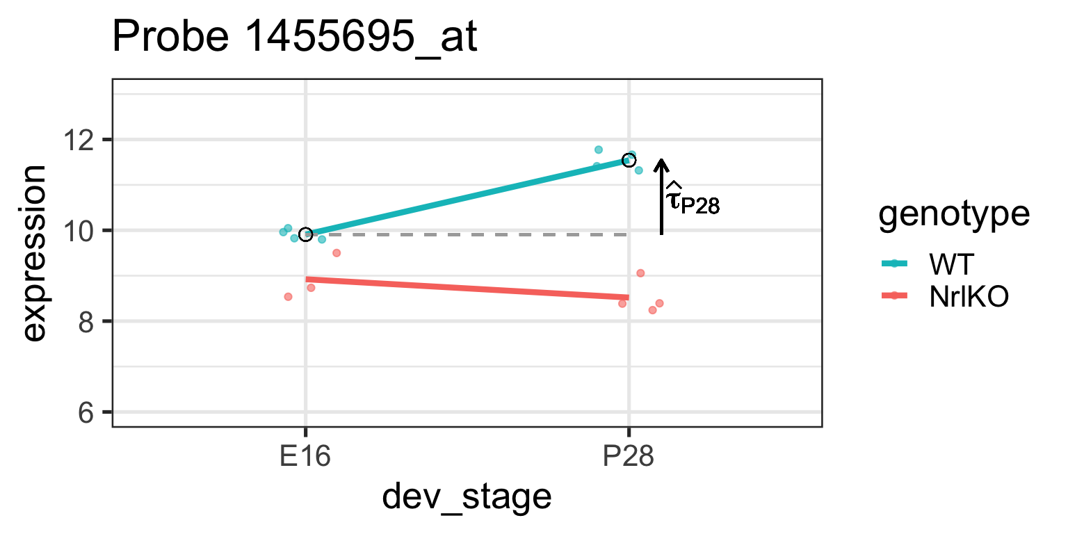
And now the “treatment effects”…

Important: Simple/Conditional vs Main/Marginal effects

“Treatment effect” parameters represent conditional effects: effects at a given level of the other factor (e.g. effect of genotype at E16). These are also called simple effects. They do not represent marginal effects.

A marginal effect, on the other hand, is the overall effect of a factor, averaged over all levels of the other factor (e.g. the overall effect of genotype, averaged over all levels of developmental time). These are also called main effects.

Simple genotype effect: WT vs NrlKO at E16

Effect of genotype at E16: \(\tau_{KO}=E[Y_{NrlKO,E16}]-E[Y_{WT,E16}]\)

lm estimate: \(\hat{\tau}_{KO}\) is the difference of sample respective means (check below)

tidy(twoFactFit)

# A tibble: 4 × 5
  term                       estimate std.error statistic  p.value
  <chr>                         <dbl>     <dbl>     <dbl>    <dbl>
1 (Intercept)                   9.91      0.157     62.9  2.02e-15
2 genotypeNrlKO                -0.984     0.240     -4.09 1.78e- 3
3 dev_stageP28                  1.64      0.223      7.35 1.44e- 5
4 genotypeNrlKO:dev_stageP28   -2.04      0.328     -6.23 6.47e- 5

means.2Fact

# A tibble: 4 × 5
  dev_stage genotype cellMeans txEffects  lmEst
  <fct>     <fct>        <dbl>     <dbl>  <dbl>
1 E16       WT            9.91     0      9.91 
2 E16       NrlKO         8.92    -0.984 -0.984
3 P28       WT           11.5      1.64   1.64 
4 P28       NrlKO         8.52    -1.39  -2.04

But, do you want to test the conditional effect at E16: \(H_0: \tau_{KO}=0\)??

Simple developmental effect: E16 vs P28 in WT

Similarly, for the other factor: \(\tau_{P28}\) is the effect of developmental time (P28 vs E16) in WT

If \(\tau_{P28}=0\), what would the mean be in the WT group at P28?

Simple developmental effect: E16 vs P28 in WT

Similarly, for the other factor: \(\tau_{P28}\) is the effect of developmental time (P28 vs E16) in WT

If \(\tau_{P28}=0\), what would the mean be in the WT group at P28?

Simple developmental effect: E16 vs P28 in WT

Effect of development in WT: \(\tau_{P28}=E[Y_{WT,P28}]-E[Y_{WT,E16}]\)

lm estimate: \(\hat{\tau}_{P28}\) is the difference of respective sample means (check below)

tidy(twoFactFit)

# A tibble: 4 × 5
  term                       estimate std.error statistic  p.value
  <chr>                         <dbl>     <dbl>     <dbl>    <dbl>
1 (Intercept)                   9.91      0.157     62.9  2.02e-15
2 genotypeNrlKO                -0.984     0.240     -4.09 1.78e- 3
3 dev_stageP28                  1.64      0.223      7.35 1.44e- 5
4 genotypeNrlKO:dev_stageP28   -2.04      0.328     -6.23 6.47e- 5

means.2Fact

# A tibble: 4 × 5
  dev_stage genotype cellMeans txEffects  lmEst
  <fct>     <fct>        <dbl>     <dbl>  <dbl>
1 E16       WT            9.91     0      9.91 
2 E16       NrlKO         8.92    -0.984 -0.984
3 P28       WT           11.5      1.64   1.64 
4 P28       NrlKO         8.52    -1.39  -2.04

Again, do you want to test the conditional effect in WT: \(H_0: \tau_{P28}=0\)??

Interaction effect

Is the effect of genotype the same at different developmental stages?

Equivalently: Is the development effect the same for both genotypes?

Interaction effect

Is the effect of genotype the same at different developmental stages?

Equivalently: Is the development effect the same for both genotypes?

Interaction effect

Is the effect of genotype the same at different developmental stages?

Equivalently: Is the development effect the same for both genotypes?

Interaction effect

The genotype effect at E16 is \(\tau_{KO}\). However, \(\tau_{KO}\) does not seem to be the effect at P28.

The difference is the interaction effect! If there’s no interaction effect, \(\tau_{KO:P28}=0\)

Interaction effect

Difference of differences:

\[\tau_{KO:P28}= (E[Y_{NrlKO,P28}]-E[Y_{WT,P28}]) - (E[Y_{NrlKO,E16}]-E[Y_{WT,E16}])\]

In lm output:

tidy(twoFactFit)

# A tibble: 4 × 5
  term                       estimate std.error statistic  p.value
  <chr>                         <dbl>     <dbl>     <dbl>    <dbl>
1 (Intercept)                   9.91      0.157     62.9  2.02e-15
2 genotypeNrlKO                -0.984     0.240     -4.09 1.78e- 3
3 dev_stageP28                  1.64      0.223      7.35 1.44e- 5
4 genotypeNrlKO:dev_stageP28   -2.04      0.328     -6.23 6.47e- 5

means.2Fact

# A tibble: 4 × 5
  dev_stage genotype cellMeans txEffects  lmEst
  <fct>     <fct>        <dbl>     <dbl>  <dbl>
1 E16       WT            9.91     0      9.91 
2 E16       NrlKO         8.92    -0.984 -0.984
3 P28       WT           11.5      1.64   1.64 
4 P28       NrlKO         8.52    -1.39  -2.04

(means.2Fact$cellMeans[4] - means.2Fact$cellMeans[3]) - (means.2Fact$cellMeans[2] - means.2Fact$cellMeans[1])

[1] -2.040372

Summary of model parameters: with interaction

model parameter	`lm` estimate	stats
\(\theta\)	`(Intercept)`	\(E[Y_{WT,E16}]\)
\(\tau_{KO}\)	`genotypeNrlKO`	\(E[Y_{NrlKO,E16}] - E[Y_{WT,E16}]\)
\(\tau_{P28}\)	`dev_stageP28`	\(E[Y_{WT,P28}] - E[Y_{WT,E16}]\)
\(\tau_{KO:P28}\)	`genotypeNrlKO:dev_stageP28`	\(E[Y_{NrlKO,P28}] - E[Y_{WT,P28}] - \tau_{KO}\)

It is important to remember that lm reports simple, not main effects!

Why? Because of the parameterization used! (see companion notes)

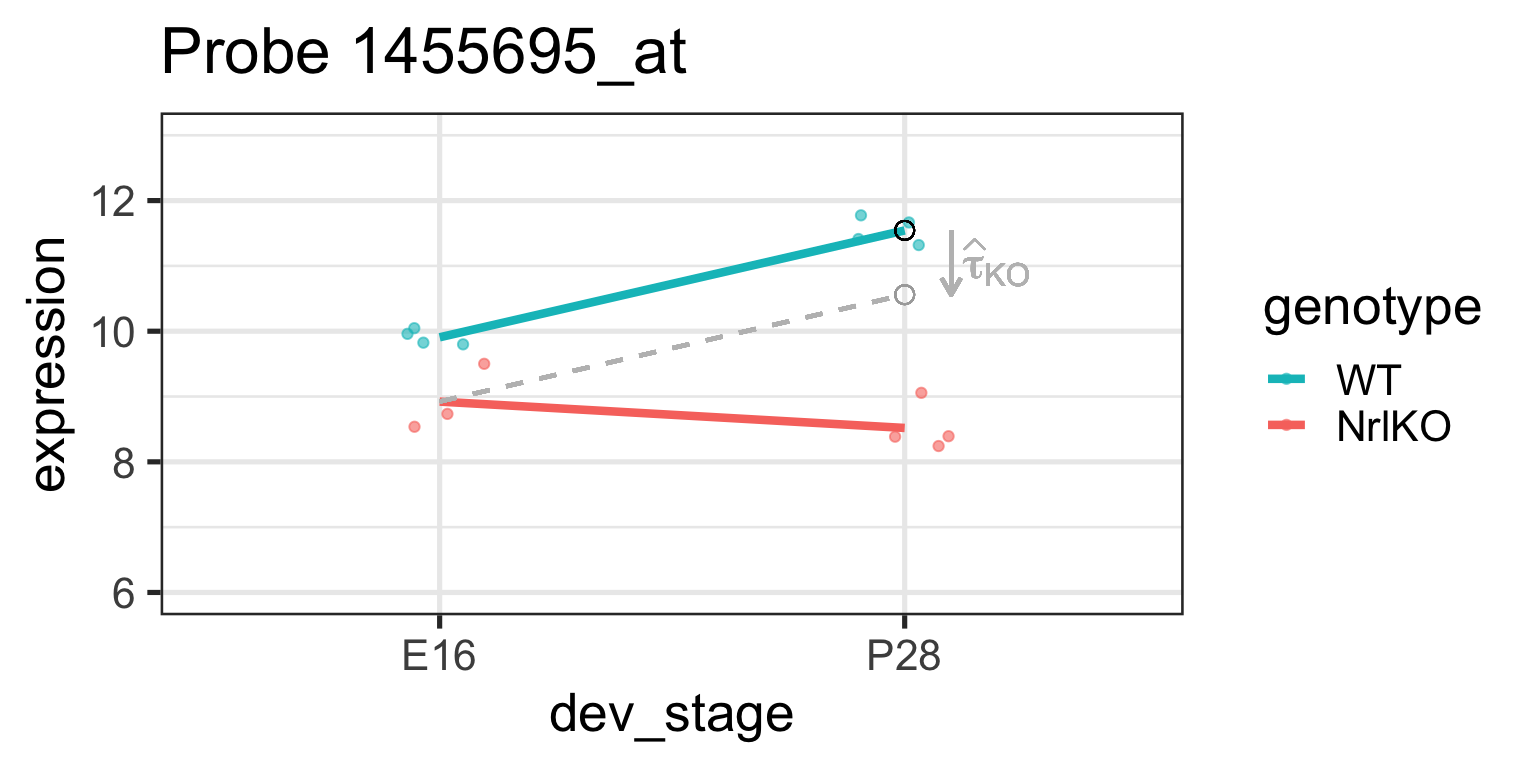
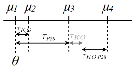
It can also be shown that \(\tau_{KO:P28}=E[Y_{NrlKO,P28}]-\tau_{P28}-\tau_{KO}-\theta\) (see previous slide and companion notes)

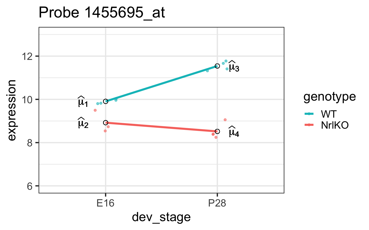
Let’s examine these parameters closer

For our model, lm tests 4 hypotheses:

\(H_0: \theta=0\)

\(H_0: \tau_{KO}=0\)

\(H_0: \tau_{P28}=0\)

\(H_0: \tau_{KO:P28}=0\)

We may not be interested in these hypotheses, e.g., \(\tau_{KO}\) and \(\tau_{P28}\) are conditional effects at a given level of a factor (simple effects)

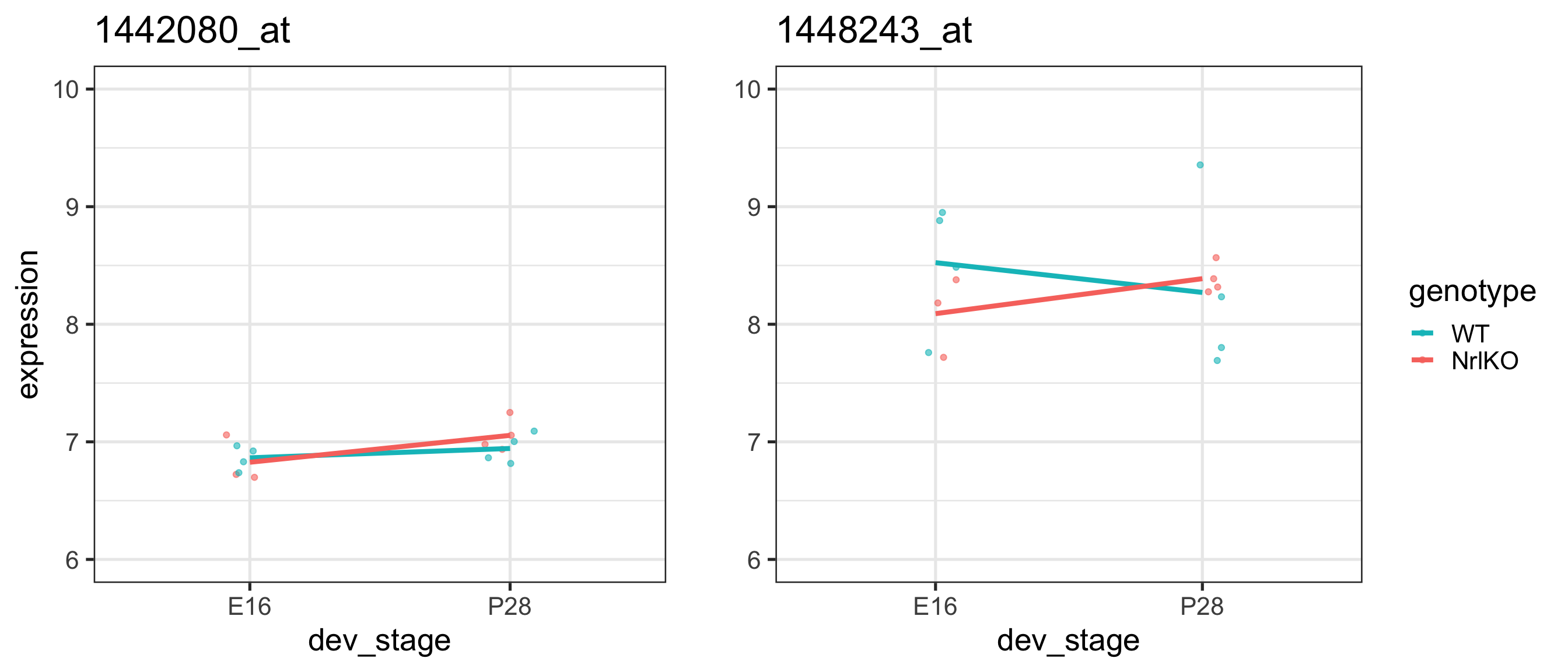
Ex 1: nothing statistically significant, very flat genes

Plots
lm output

filter(twoGenes, gene == "1442080_at") %>%
  lm(expression ~ genotype * dev_stage, data = .) %>%
  tidy()

# A tibble: 4 × 5
  term                       estimate std.error statistic  p.value
  <chr>                         <dbl>     <dbl>     <dbl>    <dbl>
1 (Intercept)                  6.86      0.0703    97.7   1.61e-17
2 genotypeNrlKO               -0.0378    0.107     -0.352 7.32e- 1
3 dev_stageP28                 0.0795    0.0994     0.800 4.41e- 1
4 genotypeNrlKO:dev_stageP28   0.149     0.146      1.02  3.29e- 1

filter(twoGenes, gene == "1448243_at") %>%
  lm(expression ~ genotype * dev_stage, data = .) %>%
  tidy()

# A tibble: 4 × 5
  term                       estimate std.error statistic  p.value
  <chr>                         <dbl>     <dbl>     <dbl>    <dbl>
1 (Intercept)                   8.52      0.256    33.3   2.16e-12
2 genotypeNrlKO                -0.434     0.391    -1.11  2.91e- 1
3 dev_stageP28                 -0.253     0.362    -0.700 4.99e- 1
4 genotypeNrlKO:dev_stageP28    0.551     0.533     1.03  3.24e- 1

Ex 2: statistically significant interaction (non-parallel)

Plots
lm output

filter(twoGenes, gene == "1434709_at") %>%
  lm(expression ~ genotype * dev_stage, data = .) %>%
  tidy()

# A tibble: 4 × 5
  term                       estimate std.error statistic  p.value
  <chr>                         <dbl>     <dbl>     <dbl>    <dbl>
1 (Intercept)                    8.59     0.221     38.8  4.08e-13
2 genotypeNrlKO                 -1.59     0.338     -4.71 6.43e- 4
3 dev_stageP28                  -2.22     0.313     -7.09 2.02e- 5
4 genotypeNrlKO:dev_stageP28     4.97     0.461     10.8  3.48e- 7

filter(twoGenes, gene == "1458220_at") %>%
  lm(expression ~ genotype * dev_stage, data = .) %>%
  tidy()

# A tibble: 4 × 5
  term                       estimate std.error statistic  p.value
  <chr>                         <dbl>     <dbl>     <dbl>    <dbl>
1 (Intercept)                    9.47     0.185     51.2  1.94e-14
2 genotypeNrlKO                 -2.33     0.283     -8.23 4.97e- 6
3 dev_stageP28                  -1.37     0.262     -5.24 2.75e- 4
4 genotypeNrlKO:dev_stageP28     1.51     0.385      3.92 2.40e- 3

Disagreement in simple effects with interaction

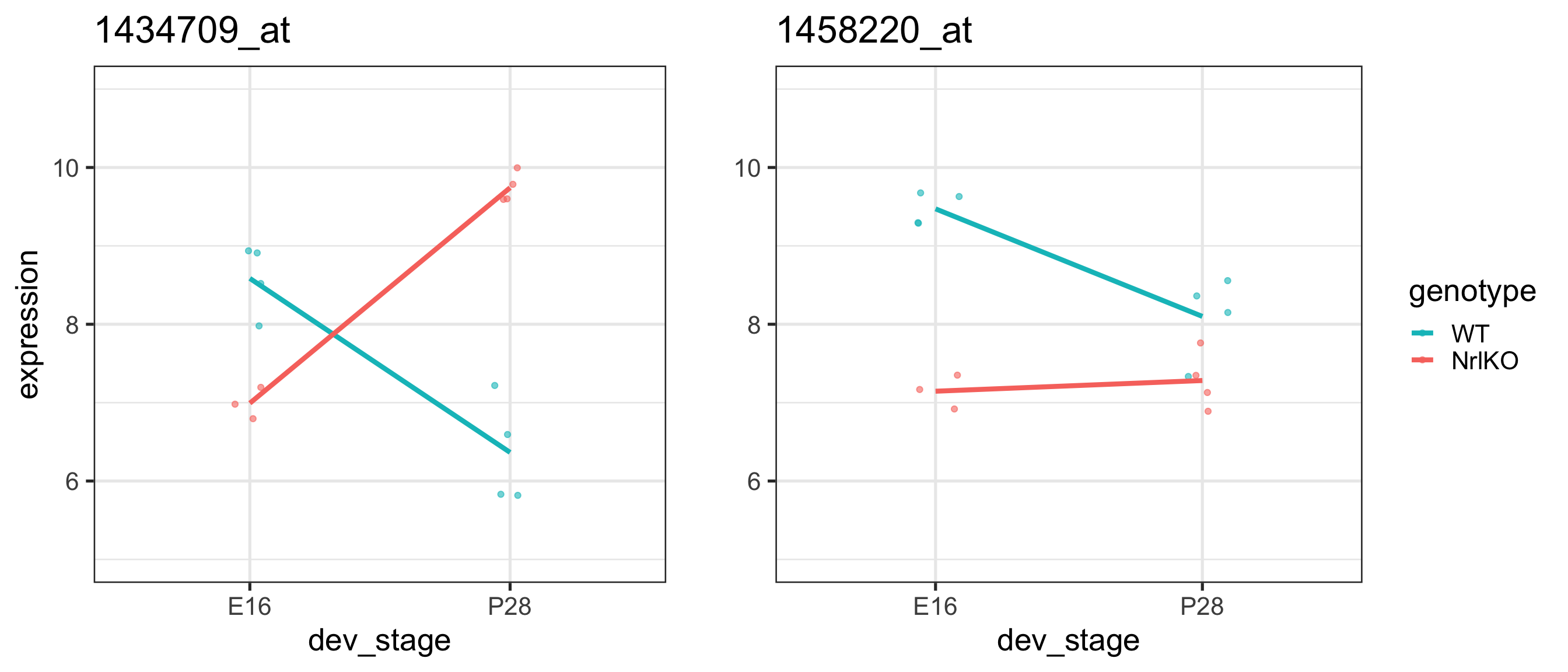
Note that a significant interaction means the simple effects may not agree
For the gene 1434709_at on the previous slide, compare the effect of genotype at E16 and P28:

Effect	`lm` output	Estimate
Genotype at E16	`genotypeNrlKO`
Genotype at P28

Main effects (overall): does genotype have an effect on gene expression?
- We can’t (yet) answer this question! It depends (on the level of dev_stage)! (more later)

Ex 3: BALANCED & only genotype at E16 is significant

For simplicity here, we’ll add a fake observation in the NrlKO & E16 group (close to its mean) so that we have a balanced design

Note

In unbalanced designs the main effects are a weighted average of the simple effects, and the weights are not easy to interpret (beyond the scope of this course but worth noting the issue!)

# recall our unbalanced design
table(pData(eset)$genotype, pData(eset)$dev_stage)

       
        E16 P2 P6 P10 P28
  WT      4  4  4   4   4
  NrlKO   3  4  4   4   4

# Duplicate sample GSM92615 (E16 NrlKO) and add noise expression
twoGenes <- filter(twoGenes, sample_id == "GSM92615") %>%
  mutate(expression = expression + rnorm(n(), 0, 0.05)) %>%
  rbind(twoGenes)

Ex 3: BALANCED & only genotype at E16 is significant

Plots
lm output

filter(twoGenes, gene == "1447753_at") %>%
  lm(expression ~ genotype * dev_stage, data = .) %>%
  tidy()

# A tibble: 4 × 5
  term                       estimate std.error statistic  p.value
  <chr>                         <dbl>     <dbl>     <dbl>    <dbl>
1 (Intercept)                  6.48      0.0454    143.   9.31e-21
2 genotypeNrlKO                0.300     0.0641      4.68 5.35e- 4
3 dev_stageP28                -0.0768    0.0641     -1.20 2.54e- 1
4 genotypeNrlKO:dev_stageP28  -0.113     0.0907     -1.24 2.38e- 1

filter(twoGenes, gene == "1431651_at") %>%
  lm(expression ~ genotype * dev_stage, data = .) %>%
  tidy()

# A tibble: 4 × 5
  term                       estimate std.error statistic  p.value
  <chr>                         <dbl>     <dbl>     <dbl>    <dbl>
1 (Intercept)                 6.50       0.0710   91.6    1.92e-18
2 genotypeNrlKO               0.220      0.100     2.19   4.88e- 2
3 dev_stageP28               -0.00250    0.100    -0.0249 9.81e- 1
4 genotypeNrlKO:dev_stageP28 -0.105      0.142    -0.736  4.76e- 1

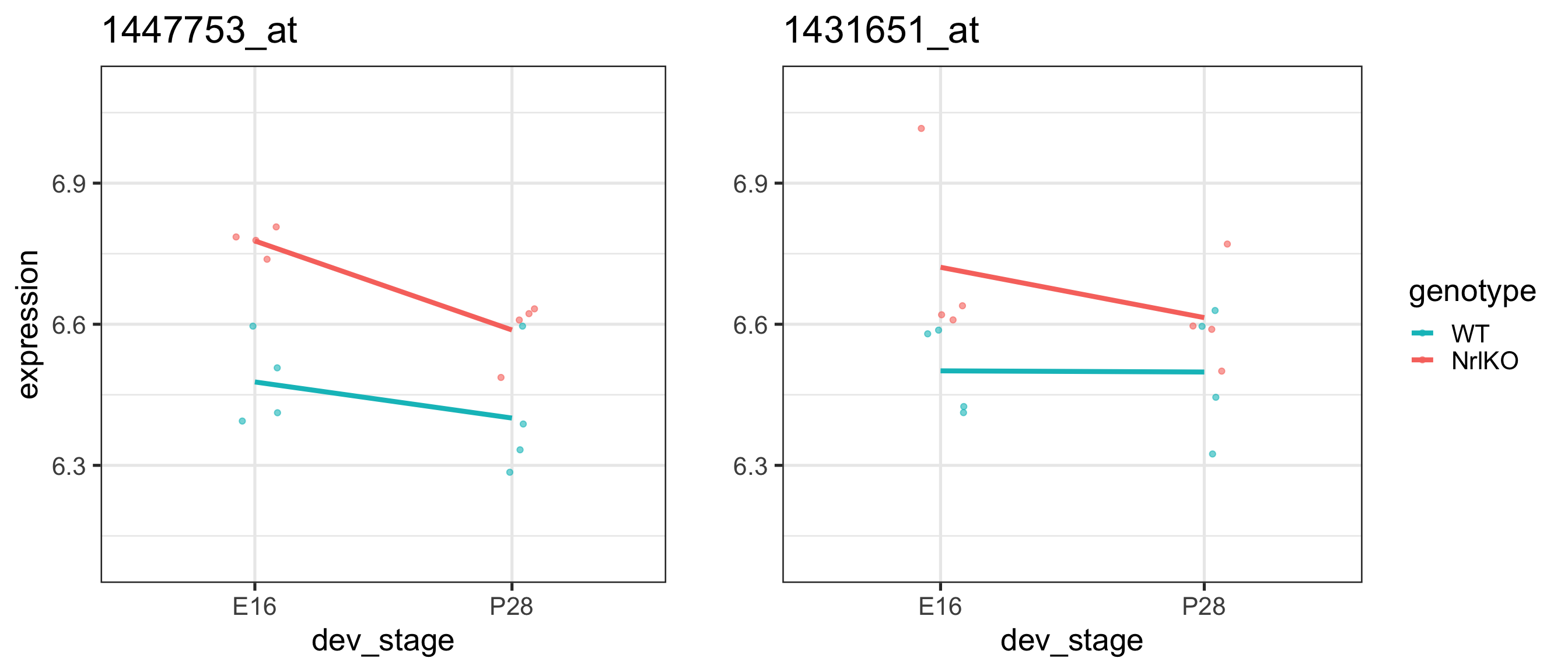
Ex 3: BALANCED & only genotype at E16 is significant

For both of these genes:

The interaction effect is not significant (almost parallel pattern)
The effect of developmental stage is not significant for WT (almost flat pattern)
There is a significant genotype effect at E16
There may be a genotype effect regardless of the developmental stage (main effect). However, that hypothesis is not tested here!!

How do we test a main effect??

How do we test for a main effect?

The main effect measures the overall association between the response and a factor - it is the (weighted) average of an effect over the levels of the other factor
anova() can be used to test the main effects
The following is the null hypothesis that there is no main effect of genotype:

\[H_0: \frac{(E[Y_{KO,E16}]-E[Y_{WT,E16}])+(E[Y_{KO,P28}]-E[Y_{WT,P28}])}{2}=0\]

Note

For unbalanced experiments \(H_0: w_1 \text{effect}_{E16}+ w_2 \text{effect}_{P28}=0\), where \(w_1\) and \(w_2\) are sample size weights

Main effects using `anova`

filter(twoGenes, gene == "1447753_at") %>%
  lm(expression ~ genotype * dev_stage, data = .) %>%
  anova() %>% 
  tidy()

# A tibble: 4 × 6
  term                  df  sumsq  meansq statistic   p.value
  <chr>              <int>  <dbl>   <dbl>     <dbl>     <dbl>
1 genotype               1 0.237  0.237       28.8   0.000168
2 dev_stage              1 0.0709 0.0709       8.62  0.0125  
3 genotype:dev_stage     1 0.0127 0.0127       1.54  0.238   
4 Residuals             12 0.0987 0.00823     NA    NA

As we suspected, there is a significant genotype effect for this probe (1447753_at), i.e., its mean expression changes in NrlKO group (compared to WT), on average over developmental stages.

Technical note:

anova() uses type I sums of squares (sequential; conditional on previous terms), thus order matters in unbalanced designs! See this primer on types of sums of squares for an intuitive explanation.

Main & interaction effects: important notes

A significant interaction effect means that the effect of one factor depends on the levels of another
- e.g., the effect of genotype depends on developmental stage
Main effects: are the (weighted) average of an effect over the levels of the other factor
A non-significant main effect means that, on average, there’s no evidence of a factor’s effect
- e.g., no evidence of a genotype effect, on average over both developmental stages

Caution

If the interaction is significant, it is possible that one or both simple effects are significant but the average effect (i.e., the main effect) is not. This is because the effect of a factor depends on the level of the other one. Looking at main effects alone may mask interesting results!

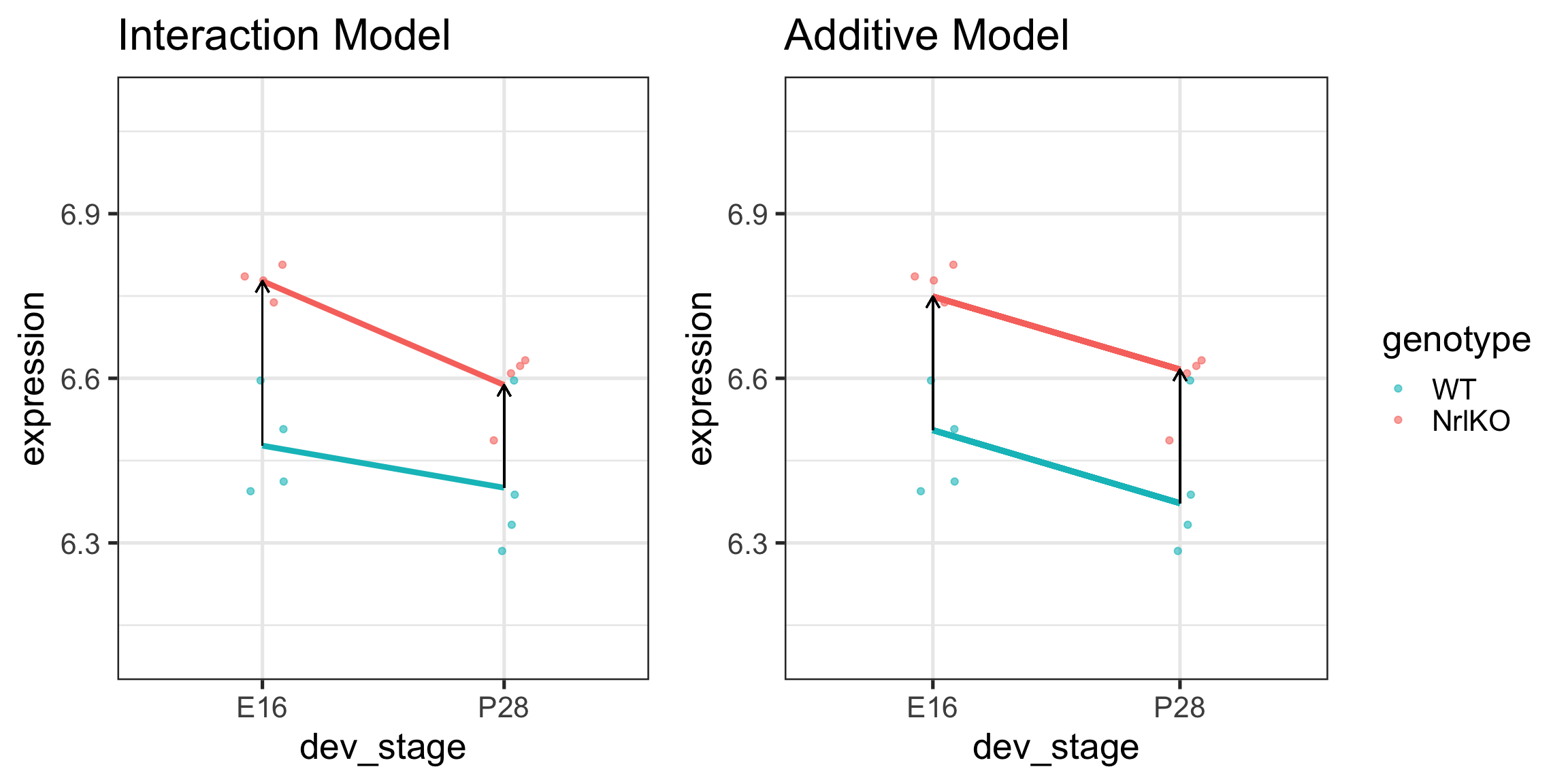
Additive models

In some applications, we need to/want to test the interaction term
However, additive models are simpler and smaller
If there are no statistical or biological grounds to include the interaction term, additive models are preferred
Additive effects: \(E[Y_{NrlKO,P28}]-E[Y_{WT,E16}]=\tau_{KO}+\tau_{P28}\)

filter(twoGenes, gene == "1447753_at") %>%
  lm(expression ~ genotype + dev_stage, data = .) %>%
  tidy()

# A tibble: 3 × 5
  term          estimate std.error statistic  p.value
  <chr>            <dbl>     <dbl>     <dbl>    <dbl>
1 (Intercept)      6.51     0.0401    162.   6.96e-23
2 genotypeNrlKO    0.244    0.0463      5.26 1.54e- 4
3 dev_stageP28    -0.133    0.0463     -2.88 1.30e- 2

Check for yourself!

Note the agreement between genotypeNrlKO in this (balanced) additive model, and the calculation of the main effect of genotype on slide 40 using the output of the (balanced) interaction model estimates on slide 38!

Additive models and balanced designs

In an additive model, the lm() parameters for balanced designs are average effects, over the levels of the other factor - same as in anova()!
- Note the agreement between lm and anova; this is gone in unbalanced designs since weights are computed differently!
The intercept parameter is now \(\bar{Y} - \bar{x}_{ij,KO}\hat{\tau}_{KO} - \bar{x}_{ij,P28}\hat{\tau}_{P28}\)

Note

Type III sum of squares (partial; conditional on all other terms in the model) are required for agreement in unbalanced designs (use car::Anova() to obtain) - beyond our scope

Parameters in additive models represent main effects

(fit <- filter(twoGenes, gene == "1447753_at") %>%
  lm(expression ~ genotype + dev_stage, data = .)) %>%
  tidy()

# A tibble: 3 × 5
  term          estimate std.error statistic  p.value
  <chr>            <dbl>     <dbl>     <dbl>    <dbl>
1 (Intercept)      6.51     0.0401    162.   6.96e-23
2 genotypeNrlKO    0.244    0.0463      5.26 1.54e- 4
3 dev_stageP28    -0.133    0.0463     -2.88 1.30e- 2

tidy(fit)$statistic[2]^2

[1] 27.69005

fit %>% anova() %>% tidy()

# A tibble: 3 × 6
  term         df  sumsq  meansq statistic   p.value
  <chr>     <int>  <dbl>   <dbl>     <dbl>     <dbl>
1 genotype      1 0.237  0.237       27.7   0.000154
2 dev_stage     1 0.0709 0.0709       8.27  0.0130  
3 Residuals    13 0.111  0.00857     NA    NA

Additive vs interaction models

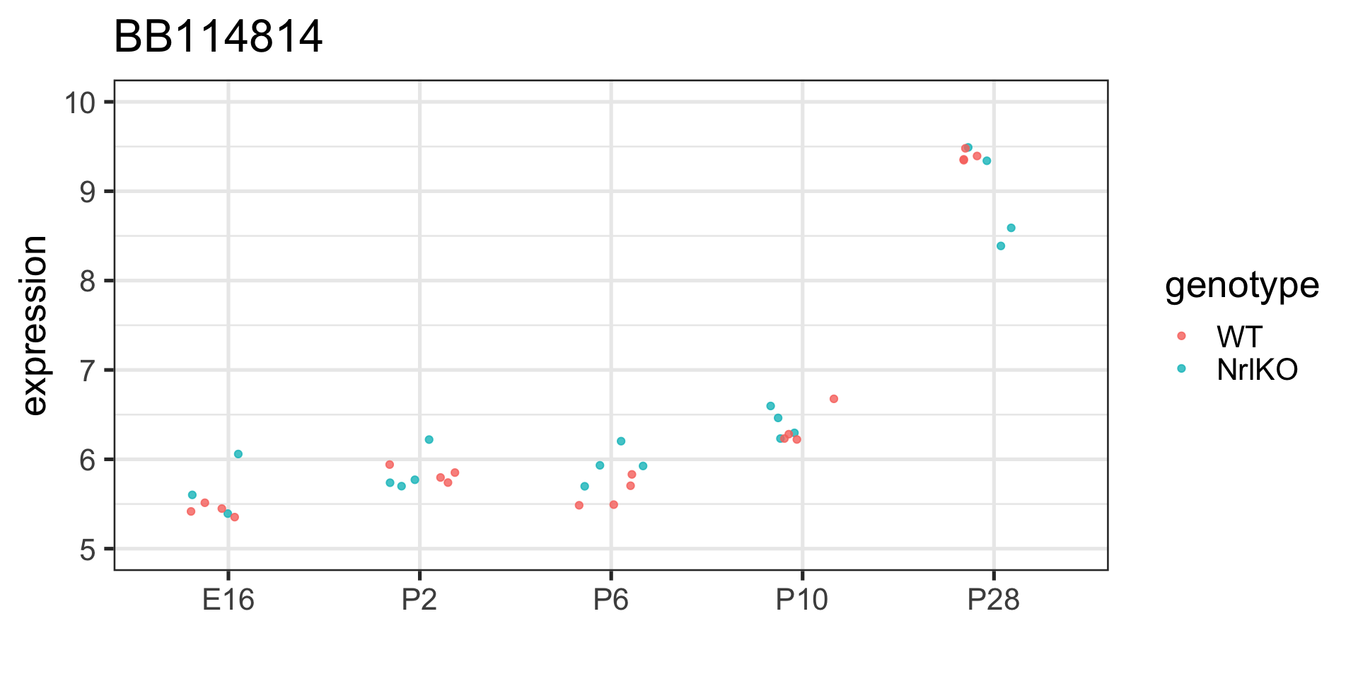
Interactions with multi-level factors (more than 2 groups)

Back to our old friend the BB114814 gene

Interactions with multi-level factors (more than 2 groups)

We can generalize the regression model to factors with more levels (e.g., E16, P2, P10 and P28): we just add more indicator variables (and parameters)!

With interaction

Code

bb1gene <- toLongerMeta(eset) %>% 
  filter(gene %in% c("1440645_at")) %>%
  mutate(gene = "BB114814")

(itxFit <- lm(expression ~ genotype*dev_stage, data = bb1gene)) %>%
  tidy()

# A tibble: 10 × 5
   term                       estimate std.error statistic  p.value
   <chr>                         <dbl>     <dbl>     <dbl>    <dbl>
 1 (Intercept)                  5.43       0.124    43.8   4.76e-28
 2 genotypeNrlKO                0.252      0.189     1.33  1.95e- 1
 3 dev_stageP2                  0.399      0.175     2.27  3.05e- 2
 4 dev_stageP6                  0.195      0.175     1.11  2.75e- 1
 5 dev_stageP10                 0.920      0.175     5.24  1.29e- 5
 6 dev_stageP28                 3.96       0.175    22.6   5.97e-20
 7 genotypeNrlKO:dev_stageP2   -0.226      0.258    -0.877 3.88e- 1
 8 genotypeNrlKO:dev_stageP6    0.0599     0.258     0.232 8.18e- 1
 9 genotypeNrlKO:dev_stageP10  -0.208      0.258    -0.804 4.28e- 1
10 genotypeNrlKO:dev_stageP28  -0.694      0.258    -2.69  1.18e- 2

Note

All the dev_stage parameters are still simple effects, but we now have more: one for each level compared to the reference

Factors with multiple levels (cont.)

Without interaction: additive

(addFit <- lm(expression ~ genotype + dev_stage, data = bb1gene)) %>%
  tidy()

# A tibble: 6 × 5
  term          estimate std.error statistic  p.value
  <chr>            <dbl>     <dbl>     <dbl>    <dbl>
1 (Intercept)     5.53      0.110     50.2   9.62e-33
2 genotypeNrlKO   0.0317    0.0878     0.361 7.21e- 1
3 dev_stageP2     0.302     0.142      2.13  4.11e- 2
4 dev_stageP6     0.241     0.142      1.70  9.87e- 2
5 dev_stageP10    0.832     0.142      5.86  1.44e- 6
6 dev_stageP28    3.63      0.142     25.6   2.43e-23

Parameters are now main effects (on average over the levels of the other factor), but we have more!

Question

Does developmental stage have a significant effect on this gene’s expression?

We haven’t tested that!!

Recall: F-test and overall significance

the t-test in linear regression allows us to test single hypotheses; these are given in the summary of lm \[H_0 : \tau_i = 0\] \[H_A : \tau_j \neq 0\]
but we often like to test multiple hypotheses simultaneously: \[H_0 : \tau_{P2} = \tau_{P6} = \tau_{P10} = \tau_{P28}=0\textrm{ [AND statement]}\] \[H_A : \tau_j \neq 0 \textrm{ for at least one j [OR statement]}\] the F-test allows us to test such compound tests

Overall effects: compound tests

Interaction model with two factors: genotype and (5-level) developmental time

lm output tests the following null hypotheses (OR):

\(H_0: \tau_{KO}=0\) (1 df)
\(H_0: \tau_{P2}=\tau_{P6}=\tau_{P10}=\tau_{P28}=0\) (in WT!, 4 df)
\(H_0: \tau_{KO:P2}=\tau_{KO:P6}=\tau_{KO:P10}=\tau_{KO:P28}=0\) (4 df)

anova output: tests overall effects of a factor (AND) controlling for the previous ones

anova(itxFit) %>% tidy()

# A tibble: 4 × 6
  term                  df   sumsq  meansq statistic   p.value
  <chr>              <int>   <dbl>   <dbl>     <dbl>     <dbl>
1 genotype               1  0.0693  0.0693      1.13  2.97e- 1
2 dev_stage              4 71.0    17.8       288.    6.72e-23
3 genotype:dev_stage     4  0.689   0.172       2.80  4.43e- 2
4 Residuals             29  1.78    0.0616     NA    NA

Overall effects: compound tests (cont.)

Additive model with genotype and development time (5-level); no interaction

lm output tests the following null hypotheses (OR)

\(H_0: \tau_{KO}=0\) (1 df)
\(H_0: \tau_{P2}=\tau_{P6}=\tau_{P10}=\tau_{P28}=0\) (on average!, 4 df)

anova output tests overall effects of a factor (AND) controlling for the previous ones

anova(addFit) %>% tidy()

# A tibble: 3 × 6
  term         df   sumsq  meansq statistic   p.value
  <chr>     <int>   <dbl>   <dbl>     <dbl>     <dbl>
1 genotype      1  0.0693  0.0693     0.925  3.43e- 1
2 dev_stage     4 71.0    17.8      237.     8.45e-24
3 Residuals    33  2.47    0.0750    NA     NA

Note

The \(t\)-test in lm and the \(F\)-test (1 df) in anova for genotype are not equivalent here due to unbalancedness (order matters)

These examples are just special cases of nested models

For example: does development have a significant effect on gene expression?

Compare the models with and without dev_stage!

Model 1: expression ~ genotype

Model 2: expression ~ genotype + dev_stage

Mathematically:

Model 1: \(Y_{ijk}=\theta + \tau_{KO}x_{KO,ijk} + \varepsilon\)

Model 2: \(Y_{ijk}=\theta + \tau_{KO}x_{KO,ijk} + \tau_{P2}x_{P2,ijk}+\tau_{P6}x_{P6,ijk}+\tau_{P10}x_{P10,ijk}+\tau_{P28}x_{P28,ijk}+ \varepsilon\)

\[H_0: \tau_{P2}=\tau_{P6}=\tau_{P10}=\tau_{P28}=0\]

The \(x_{**,ijk}\) are indicator variables (see companion notes)

More general: F-test to compare nested models

\(H_0: \alpha_{k+1} = ... = \alpha_{k+p}\)

\[F = \frac{(SS_{reduced} - SS_{full})/(p)}{SS_{full} / (n-p-k-1)} \sim \mathbf{F}_{p, \,n-p-k-1}\] This \(F\)-statistic compares the following two models:

Reduced (k + 1 parameters): \[y_i = \alpha_0 + \alpha_1 x_{i1} + ... + \alpha_k x_{ik} + \epsilon_i\]
Full (p + k + 1 parameters): \[y_i = \alpha_0 + \alpha_1 x_{i1} + ... + \alpha_k x_{ik} + ... + \alpha_p x_{ip} + \epsilon_i\]

A significant F-statistic here means that the full model explains significantly more variation in the outcome variable than the reduced model

Nested models in R

addReduced <- lm(expression ~ genotype, data = bb1gene)
addFull <- lm(expression ~ genotype + dev_stage, data = bb1gene)
anova(addReduced,addFull)

Analysis of Variance Table

Model 1: expression ~ genotype
Model 2: expression ~ genotype + dev_stage
  Res.Df    RSS Df Sum of Sq      F    Pr(>F)    
1     37 73.497                                  
2     33  2.474  4    71.023 236.84 < 2.2e-16 ***
---
Signif. codes:  0 '***' 0.001 '**' 0.01 '*' 0.05 '.' 0.1 ' ' 1

anova(addFull) %>% tidy()

# A tibble: 3 × 6
  term         df   sumsq  meansq statistic   p.value
  <chr>     <int>   <dbl>   <dbl>     <dbl>     <dbl>
1 genotype      1  0.0693  0.0693     0.925  3.43e- 1
2 dev_stage     4 71.0    17.8      237.     8.45e-24
3 Residuals    33  2.47    0.0750    NA     NA

Another special case: overall goodness of fit!

Compare the full vs the intercept-only models (compound test)! \[H_0: \tau_{KO}=\tau_{P2}=\tau_{P6}=\tau_{P10}=\tau_{P28}=0 \, \ (5 \text{ df})\]

addReduced <- lm(expression ~ 1, data = bb1gene)
anova(addReduced,addFull)

Analysis of Variance Table

Model 1: expression ~ 1
Model 2: expression ~ genotype + dev_stage
  Res.Df    RSS Df Sum of Sq      F    Pr(>F)    
1     38 73.566                                  
2     33  2.474  5    71.092 189.66 < 2.2e-16 ***
---
Signif. codes:  0 '***' 0.001 '**' 0.01 '*' 0.05 '.' 0.1 ' ' 1

Goodness of fit also given in output of `lm`

summary(addFull)


Call:
lm(formula = expression ~ genotype + dev_stage, data = bb1gene)

Residuals:
     Min       1Q   Median       3Q      Max 
-0.80137 -0.12454 -0.03212  0.17038  0.50036 

Coefficients:
              Estimate Std. Error t value Pr(>|t|)    
(Intercept)    5.52734    0.11012  50.192  < 2e-16 ***
genotypeNrlKO  0.03167    0.08785   0.361   0.7207    
dev_stageP2    0.30152    0.14185   2.126   0.0411 *  
dev_stageP6    0.24102    0.14185   1.699   0.0987 .  
dev_stageP10   0.83185    0.14185   5.864 1.44e-06 ***
dev_stageP28   3.63011    0.14185  25.592  < 2e-16 ***
---
Signif. codes:  0 '***' 0.001 '**' 0.01 '*' 0.05 '.' 0.1 ' ' 1

Residual standard error: 0.2738 on 33 degrees of freedom
Multiple R-squared:  0.9664,    Adjusted R-squared:  0.9613 
F-statistic: 189.7 on 5 and 33 DF,  p-value: < 2.2e-16

Summary so far

t-tests can be used to test the equality of 2 population means
ANOVA can be used to test the equality of more than 2 population means simultaneously (main effects)
Linear regression provides a general framework for modelling the relationship between a response and different type of explanatory variables
- t-tests are used to test the significance of simple effects (individual coefficients)
- F-tests are used to test the significance of main effects (simultaneously multiple coefficients)
- F-tests are used to compare nested models (overall effects or goodness of fit)
Next up: continuous explanatory variables! Multiple genes!

Linear models with multiple factors

Project next steps - written proposal

Last class…

Comparing more than two groups

Quick review: from \(t\)-test to linear regression

↓

How? Why?

↓

How: Cell means model using indicator variables

How: Reference-treatment parameterization using indicator variables

How: Using matrix notation

Why: Flexible framework

Parameterizations

\[\bf{Y} = \bf{X\alpha} + \varepsilon\]

Example: compare means between groups

We can tell R to use the cell-means parameterization

Converting between parameterizations

Learning objectives for today

What if you have 2 categorical variables?

What if you have 2 categorical variables?

Two-way ANOVA (or a linear model with interaction)

Reference-treatment effect parameterization

Cell-means and treatment effects in the two-way model

What is the reference group here?

The reference: WT & E16

Simple genotype effect: WT vs NrlKO at E16

Simple genotype effect: WT vs NrlKO at E16

Simple developmental effect: E16 vs P28 in WT

Simple developmental effect: E16 vs P28 in WT

Simple developmental effect: E16 vs P28 in WT

Interaction effect

Interaction effect

Interaction effect

Interaction effect

Interaction effect

Summary of model parameters: with interaction

Let’s examine these parameters closer

\(H_0: \theta=0\)

\(H_0: \tau_{KO}=0\)

\(H_0: \tau_{P28}=0\)

\(H_0: \tau_{KO:P28}=0\)

Ex 1: nothing statistically significant, very flat genes

Ex 2: statistically significant interaction (non-parallel)

Disagreement in simple effects with interaction

Ex 3: BALANCED & only genotype at E16 is significant

Ex 3: BALANCED & only genotype at E16 is significant

Ex 3: BALANCED & only genotype at E16 is significant

How do we test for a main effect?

Main effects using anova

Main & interaction effects: important notes

Additive models

Additive models and balanced designs

Parameters in additive models represent main effects

Additive vs interaction models

Interactions with multi-level factors (more than 2 groups)

Interactions with multi-level factors (more than 2 groups)

Factors with multiple levels (cont.)

Recall: F-test and overall significance

Overall effects: compound tests

Overall effects: compound tests (cont.)

These examples are just special cases of nested models

More general: F-test to compare nested models

Nested models in R

Another special case: overall goodness of fit!

Goodness of fit also given in output of lm

Summary so far

Main effects using `anova`

Goodness of fit also given in output of `lm`