t-tests can be used to test the equality of 2 population means
ANOVA can be used to test the equality of more than 2 population means
Linear regression provides a general framework for modeling the relationship between a response variable and different types of explanatory variables
t-tests can be used to test the significance of individual coefficients
F-tests can be used to test the simultaneous significance of multiple coefficients (e.g. multiple levels of a single categorical factor, or multiple factors at once)
F-tests can be used to compare nested models (overall effects or goodness of fit)
Learning objectives for today
Understand how linear regression represents continuous variables:
Be familiar with the intuition behind how the regression line is estimated (Ordinary Least Squares)
Interpret parameters in a multiple linear regression model with continuous and factor variables
Explain the motivation behind specialized regression models in high-dimensional settings
List the advantages of the Empirical Bayes techniques in limma compared to traditional linear regression models
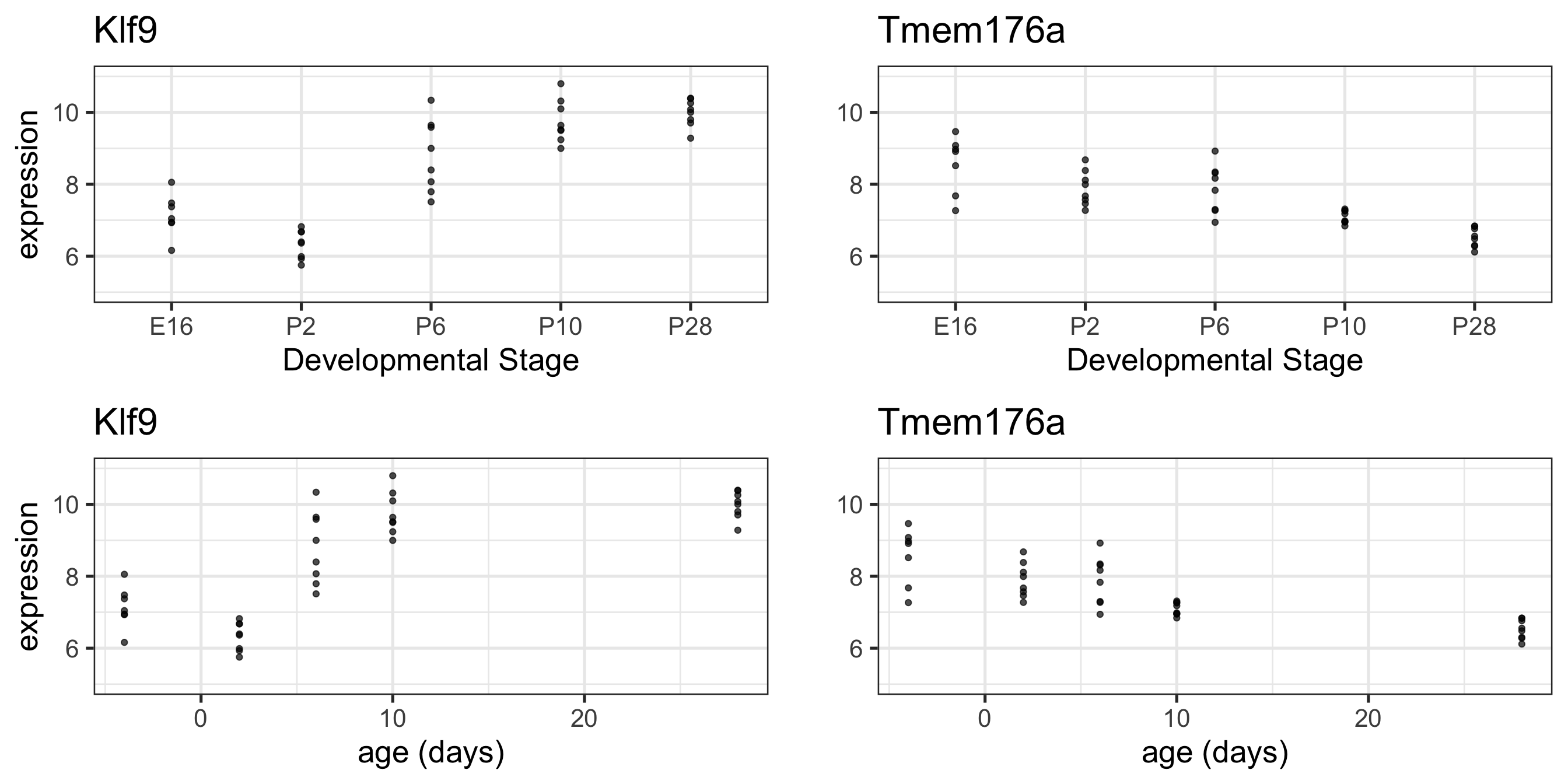
What if we treat age as a continuous variable?
Code
# read in our dataseteset <-getGEO("GSE4051", getGPL =FALSE)[[1]]# recode time pointspData(eset) <-pData(eset) %>%mutate(sample_id = geo_accession) %>%mutate(dev_stage =case_when(grepl("E16", title) ~"E16",grepl("P2", title) ~"P2",grepl("P6", title) ~"P6",grepl("P10", title) ~"P10",grepl("4 weeks", title) ~"P28" )) %>%mutate(genotype =case_when(grepl("Nrl-ko", title) ~"NrlKO",grepl("wt", title) ~"WT" ))# reorder factor levels, add continous age variablepData(eset) <-pData(eset) %>%mutate(dev_stage =fct_relevel(dev_stage, "E16", "P2", "P6", "P10", "P28")) %>%mutate(genotype =as.factor(genotype)) %>%mutate(genotype =fct_relevel(genotype, "WT", "NrlKO")) %>%mutate(age =ifelse(dev_stage =="E16", -4,ifelse(dev_stage =="P2", 2, ifelse(dev_stage =="P6", 6, ifelse(dev_stage =="P10", 10, 28)))))# function to return tidy data that merges expression matrix and metadatatoLongerMeta <-function(expset) {stopifnot(class(expset) =="ExpressionSet") expressionMatrix <- lonExpressionressionMatrix <-exprs(expset) %>%as.data.frame() %>%rownames_to_column("gene") %>%pivot_longer(cols =!gene, values_to ="expression",names_to ="sample_id") %>%left_join(pData(expset) %>%select(sample_id, dev_stage, age, genotype),by ="sample_id")return(expressionMatrix)}# pull out two genes of interesttwoGenes <-toLongerMeta(eset) %>%filter(gene %in%c("1456341_a_at", "1441811_x_at")) %>%mutate(gene =ifelse(gene =="1456341_a_at", "Klf9", "Tmem176a")) # make some plots - first with age continuousKlf9_C <-ggplot(filter(twoGenes, gene =="Klf9"), aes(x = age, y = expression)) +geom_point(alpha =0.7) +labs(title ="Klf9") +theme(legend.position ="none") +ylim(5, 11) +xlab("age (days)") Tmem176a_C <-ggplot(filter(twoGenes, gene =="Tmem176a"), aes(x = age, y = expression)) +geom_point(alpha =0.7) +labs(title ="Tmem176a") +ylim(5, 11) +xlab("age (days)") # next with age categoricalKlf9 <-ggplot(filter(twoGenes, gene =="Klf9"), aes(x = dev_stage, y = expression)) +geom_point(alpha =0.7) +theme(legend.position ="none") +labs(title ="Klf9") +ylim(5, 11) +xlab("Developmental Stage")Tmem176a <-ggplot(filter(twoGenes, gene =="Tmem176a"), aes(x = dev_stage, y = expression)) +geom_point(alpha =0.7) +labs(title ="Tmem176a") +ylim(5, 11) +xlab("Developmental Stage") grid.arrange(Klf9, Tmem176a +ylab(""), Klf9_C, Tmem176a_C +ylab(""), nrow =2)
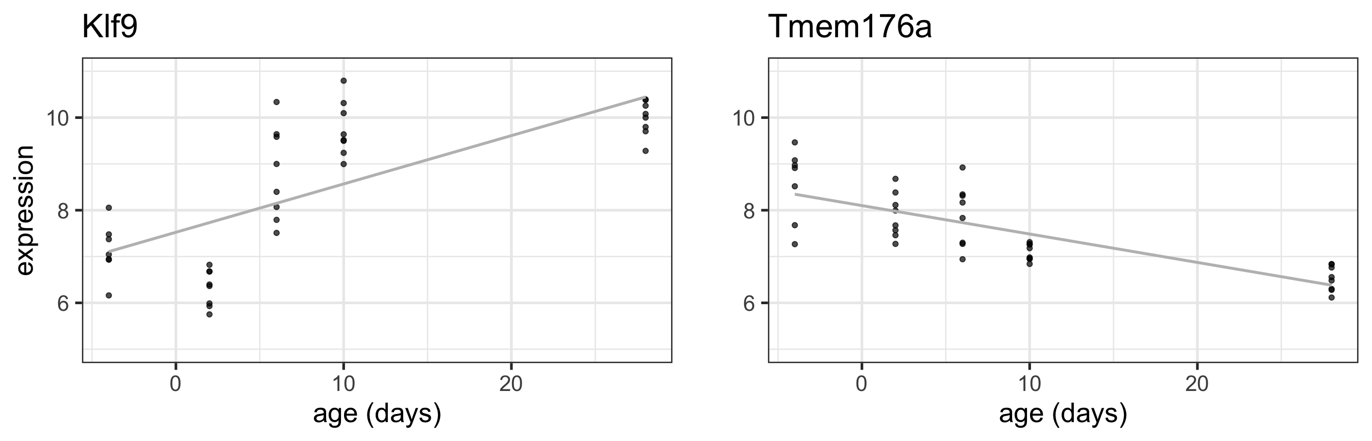
Linear model with age as continuous covariate
Code
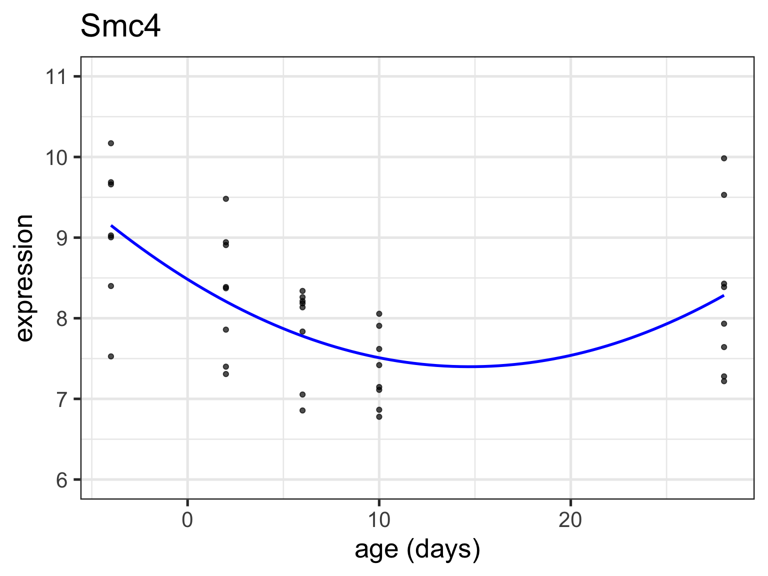
grid.arrange(Klf9_C +geom_smooth(method='lm', colour ="grey", se =FALSE), Tmem176a_C +geom_smooth(method='lm', colour ="grey", se =FALSE) +ylab(""), nrow =1)
Linear looks reasonable for gene Tmem176a, but not so much for Klf9
For now, assume linear is reasonable
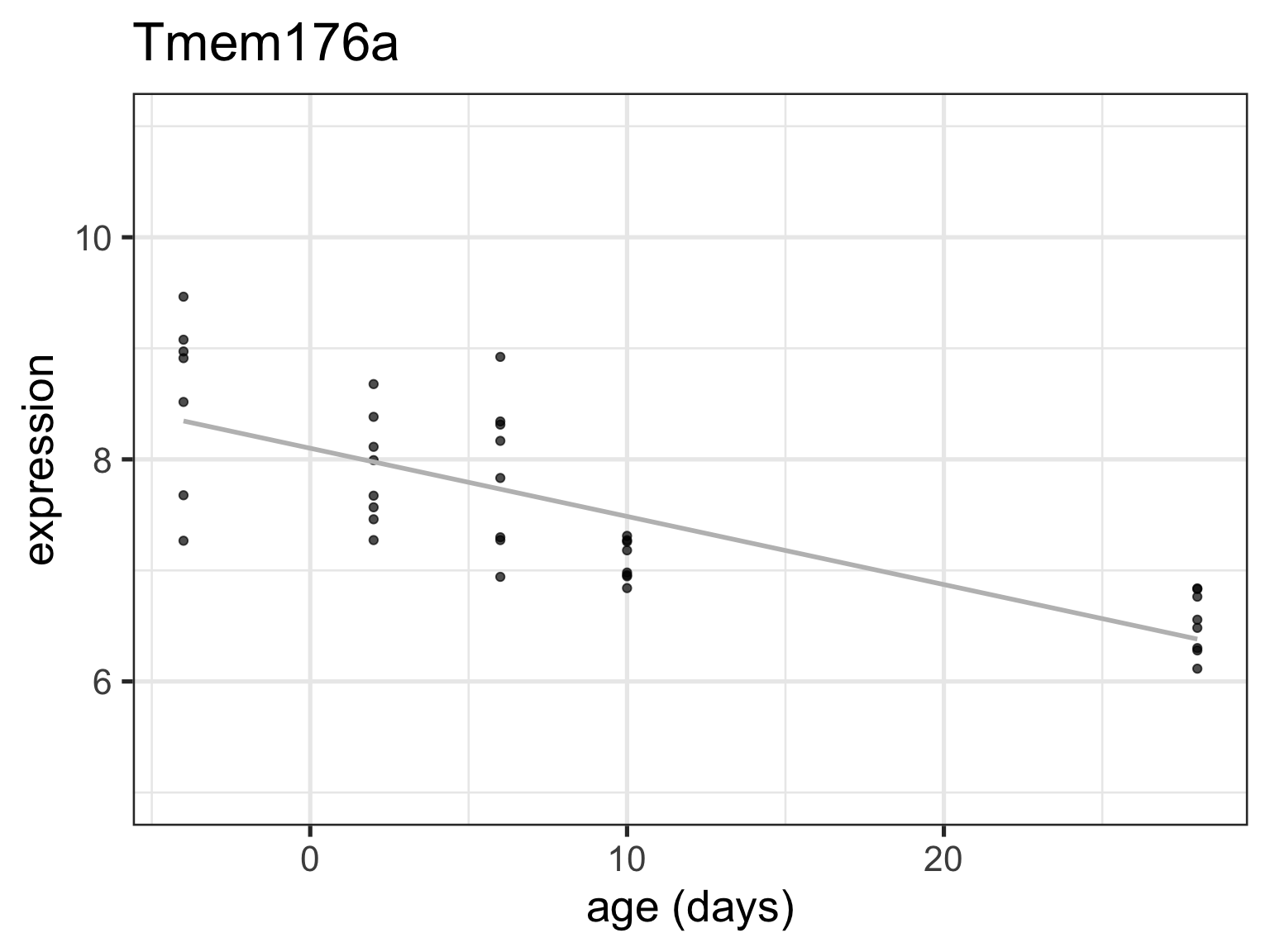
Simple Linear Regression (Matrix form)
\[ \mathbf{Y = X \boldsymbol\alpha + \boldsymbol\varepsilon}\]
Tmem_fit <-filter(twoGenes, gene =="Tmem176a") %>%lm(expression ~ age, data = .)tidy(Tmem_fit)
# A tibble: 2 × 5
  term        estimate std.error statistic  p.value
  <chr>          <dbl>     <dbl>     <dbl>    <dbl>
1 (Intercept)   8.10     0.114       71.1  3.58e-41
2 age          -0.0614   0.00821     -7.47 6.74e- 9
Interpretation of intercept:
\(H_0: \alpha_0 = 0\) tests the null hypothesis that the intercept is zero - usually, not of interest
SLR with continuous age covariate
tidy(Tmem_fit)
# A tibble: 2 × 5
  term        estimate std.error statistic  p.value
  <chr>          <dbl>     <dbl>     <dbl>    <dbl>
1 (Intercept)   8.10     0.114       71.1  3.58e-41
2 age          -0.0614   0.00821     -7.47 6.74e- 9
Interpretation of slope:
\(H_0: \alpha_1 = 0\) tests the null hypothesis that there is no association between gene expression and age - usually of interest
How do we estimate the intercept and slope?
Why is this the optimal line?
tidy(Tmem_fit)
# A tibble: 2 × 5
  term        estimate std.error statistic  p.value
  <chr>          <dbl>     <dbl>     <dbl>    <dbl>
1 (Intercept)   8.10     0.114       71.1  3.58e-41
2 age          -0.0614   0.00821     -7.47 6.74e- 9
Which one is the best line?
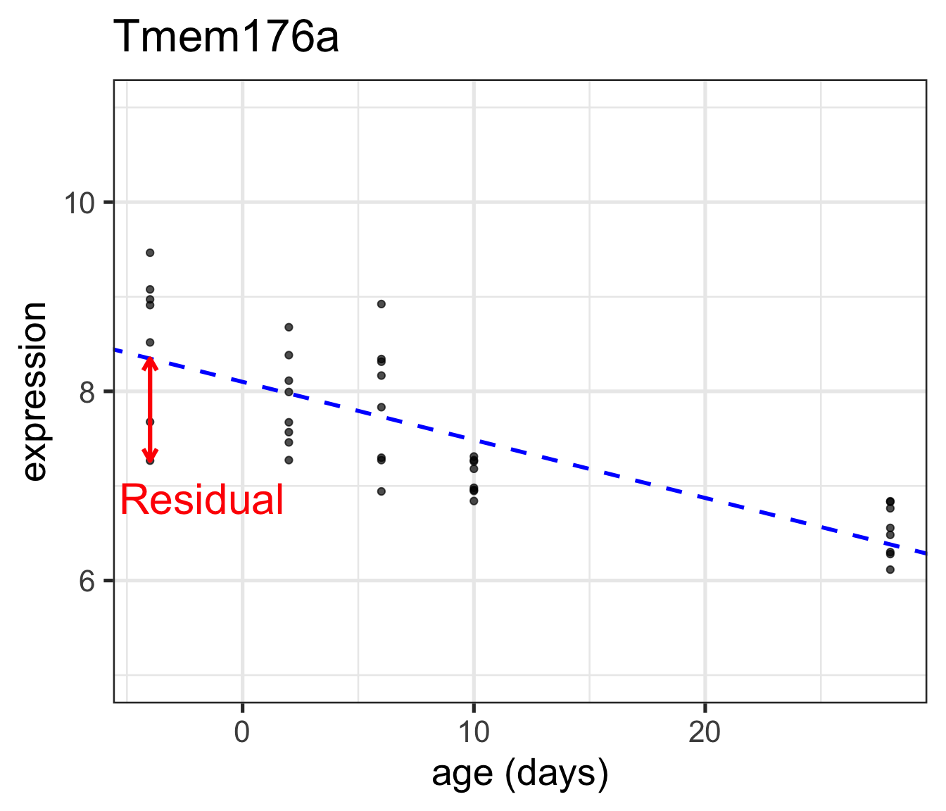
Ordinary Least Squares
Ordinary Least Squares (OLS) regression: parameter estimates minimize the sum of squared errors
Error: vertical \((y)\) distance between the true regression line (unobserved) and the real observation
Residual: vertical \((y)\) distance between the fitted regression line and the real observation (estimated error)
OLS Estimator for Simple Linear Regression (1 covariate)
Mathematically: \(\varepsilon_i\) represents the error: \(\varepsilon_i = y_i - \alpha_0 - \alpha_1x_i, i = 1, ..., n\)
We want to find the line (i.e. intercept and slope) that minimizes the sum of squared errors: \[S(\alpha_0, \alpha_1)= \sum_{i=1}^n (y_i - \alpha_0 - \alpha_1 x_i)^2\]
\(S(\alpha_0, \alpha_1)\) is called an objective function
the observed sum of squared errors is referred to as Residual Sum of Squares (RSS)
Error vs Residual
Error refers to the deviation of the observed value to the (underlying) true quantity of interest
Residual refers to the difference between the observed and estimated quantity of interest
How to obtain estimates \((\hat{\alpha}_0, \hat{\alpha}_1)\) ? Let’s look at a more general case
In the first plot, drag individual points around and observe what changes in second plot
In the second plot, adjust the slope and intercept dials - what happens to the total area of the squares in the second plot when you modify the slope and intercept from the default values?
Note that you can reset to default values by refreshing the page
Properties of OLS regression
Regression model: \(\mathbf{Y = X \boldsymbol\alpha + \boldsymbol\varepsilon}\)
where \(\mathbf{H}=\mathbf{X} (\mathbf{X}^T\mathbf{X})^{-1}\mathbf{X}^T\) is called the “hat” or projection matrix
Assumptions of OLS Regression
\(\boldsymbol\varepsilon\) have mean zero
\(\boldsymbol\varepsilon\) are iid (implies constant variance)
(only required for hypothesis testing in small sample settings)\(\boldsymbol\varepsilon\) are Normally distributed
Connection to other estimators
If \(\boldsymbol\varepsilon\) are iid Normal, then OLS estimator is also MLE (Maximum Likelihood Estimator)
Properties of OLS regression (cont’d)
Residuals: (note NOT the same as errors \(\boldsymbol\varepsilon\)) \[\hat{\boldsymbol\varepsilon} = \mathbf{y} - \hat{\mathbf{y}} = \mathbf{y} - \mathbf{X} \hat{\boldsymbol\alpha}\]
Estimated standard errors for estimated regression coefficients: \(\hat{se}(\hat{\alpha}_j)\), obtained by taking the square root of the diagonal elements of \(\hat{Var}(\hat{\boldsymbol\alpha})\)
So with a large enough sample size a p-value for this hypothesis test is obtained by computing a tail probability for the observed value of \(\hat{\alpha}_j\) from a \(t_{n-p-1}\) distribution
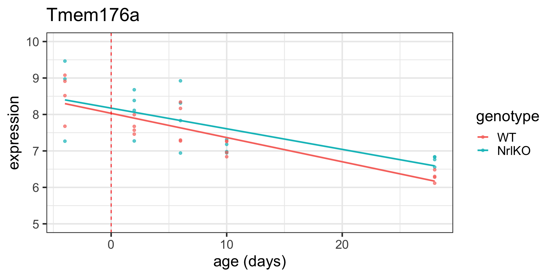
\(x_{ij, KO}\) is the indicator for WT vs KO ( \(x_{ij, KO}=1\) for \(j=NrlKO\) and 0 for \(j=WT\) )
\(x_{ij, Age}\) is the continuous age covariate
Interpretation of parameters:
\(\alpha_0\) is the expected expression in WT for age = ____
The “intercept” for the knockouts is:
The expected increase in expression in WT for every 1 day increase in age is:
The slope for the knockouts is:
Nested models
As always, you can assess the relevance of several terms at once (e.g. everything involving genotype) with an F-test:
Klf9dat <-filter(twoGenes, gene=="Klf9")anova(lm(expression ~ age*genotype, data = Klf9dat),lm(expression ~ age, data = Klf9dat))
Analysis of Variance Table

Model 1: expression ~ age * genotype
Model 2: expression ~ age
  Res.Df    RSS Df Sum of Sq      F Pr(>F)
1     35 45.948
2     37 45.984 -2 -0.036415 0.0139 0.9862
Conclusion
We don’t have evidence that genotype affects the intercept or the slope
Under \(H_0:\) the reduced model explains the same amount variation in the outcome as the full,
\[F = \frac{\frac{RSS_{Red}-RSS_{Full}}{p_{Full}-p_{Red}}}{\frac{RSS_{Full}}{n-p_{Full}-1}} \sim \text{ } F_{p_{Fill}-p_{Red},\text{ } n-{p_{Full}-1}}\] A significant F-test means we reject the null; we have evidence that the full model explains significantly more variation in the outcome than the reduced.
Collinearity & confounding
If there are problems in the experimental design, we may not be able to estimate effects of interest
Caution
The technical definition of collinearity is that a column of the design matrix can be obtained (or accurately approximated) as a linear combination of other columns.
You can think of this as one column (or variable) not containing unique information
This phenomenon can occur if our design is confounded
As an example, let’s pretend we know that all the E16 and P2 mice are female and the rest are male
Example: E16/P2 mice are female and the rest are male
# construct linear combination from columns corresponding to male timepoint indicator variablesmm[,"dev_stageP6"] + mm[,"dev_stageP10"] + mm[,"dev_stageP28"]
\(\bf{V}\) is the “unscaled covariance” matrix, and is the same for all genes!
Estimated standard errors for estimated regression coefficients: \(\large\hat{se}(\hat{\alpha}_{jg})\) obtained by taking the square root of the \(j^{th}\) diagonal element of \(\hat{Var}(\hat{\boldsymbol\alpha}_g)\), which is \(s_g\sqrt{v_{jj}}\)
What’s the big deal?
So far, nothing is new - these are the “regular” t statistics for gene g and parameter j:
\[t_{gj} = \frac{\hat{\alpha}_{gj}}{s_g \sqrt{v_{jj}}} \sim t_{d} \text{ under } H_0\]
But there are so many of them!! 😲
Observed (i.e. empirical) issues with the “standard” t-test approach for assessing differential expression
Important
Some genes with very small p-values (i.e. large -log10 p-values) are not biologically meaningful (small effect size, e.g. fold change)
How do we end up with small p-values but subtle effects?
Borrows information from all genes to get a better estimate of the variance (especially in smaller sample size settings)
Efficiently fits many regression models without replicating unnecessary calculations!
Arranges output in a convenient way to ease further analysis, visualization, and interpretation
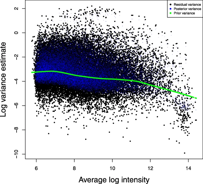
How does Empirical Bayes work?
Empirical: observed
Bayesian: incorporate ‘prior’ information
Intuition: estimate prior information from data; shrink (nudge) all estimates toward the consensus
Shrinkage = borrowing information across all genes
Genome-wide OLS fits
Gene by gene:
lm(y ~ x, data = gene) for each gene
For example, using dplyr::group_modify and broom::tidy
All genes at once, using limma:
lmFit(object, design)
object matrix-like object with expression values for all genes
design is a specially formatted design matrix (more on this later)
Note that object can be a Bioconductor container, such as an ExpressionSet object
‘Industrial scale’ model fitting is good, because computations involving just the design matrix \(\mathbf{X}\) are not repeated tens of thousands of times unnecessarily:
Under-estimated variance leads to overly large t statistic, which leads to artificially small p-value
Modeling in limma
limma assumes that for each gene \(g\) we have the following sampling distributions of the coefficient estimates and sample variances:
\[\hat{\alpha}_{gj} \,|\,\alpha_{gj}, \sigma_g^2 \sim N(\alpha_{gj}, \sigma_g^2 v_{jj})\]\[s^2_g \,|\, \sigma_g^2 \sim \frac{\sigma_g^2}{d}\chi^2_d\] These are the same as the usual assumptions about ordinary \(t\)-statistics: