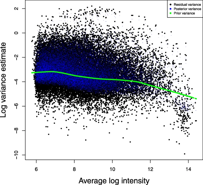
The prior parameters incorporate information from all genes which allows us to shrink/nudge the gene-specific variances toward a common consensus
they are estimated from the data - the formulas for \((s_0, d_0)\) and their derivations are beyond the scope of the course, but limma takes care of the details for us
Within each gene observations are iid / constant variance
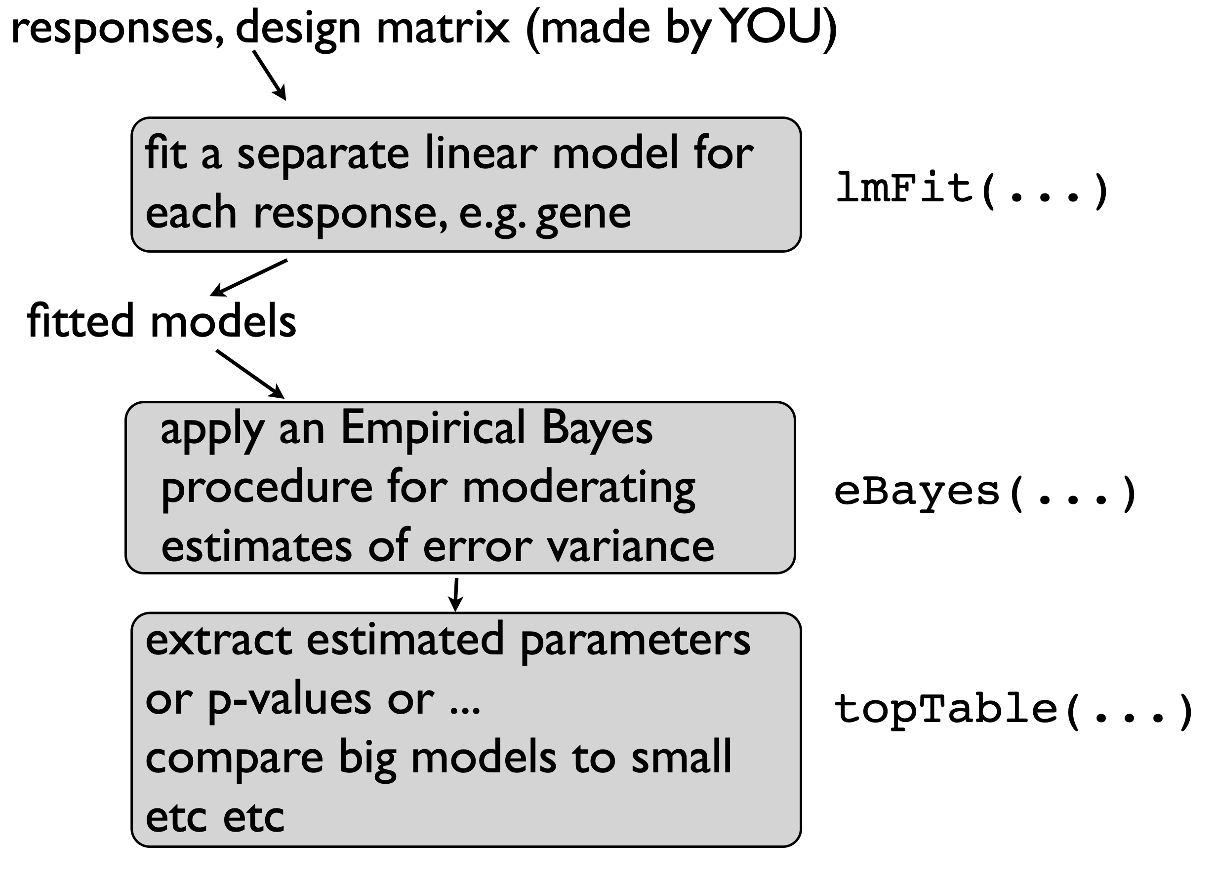
lmFit() carries out multiple linear regression on each gene
Usage: lmFit(object, design)
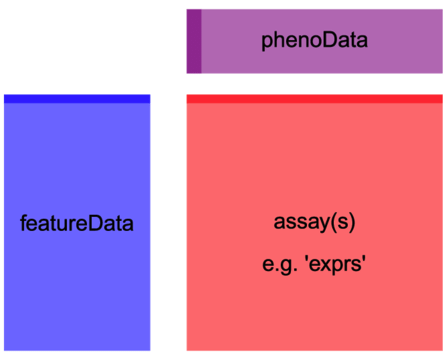
object is a data.frame or matrix with features in rows and samples in columns (G genes by N samples), or other Bioconductor object such as ExpressionSet
design is a design matrix (output of model.matrix(y ~ x); N samples by \(p+1\) parameters)
topTable(ebFit, coef = 2) is equivalent here, but much less informative!!
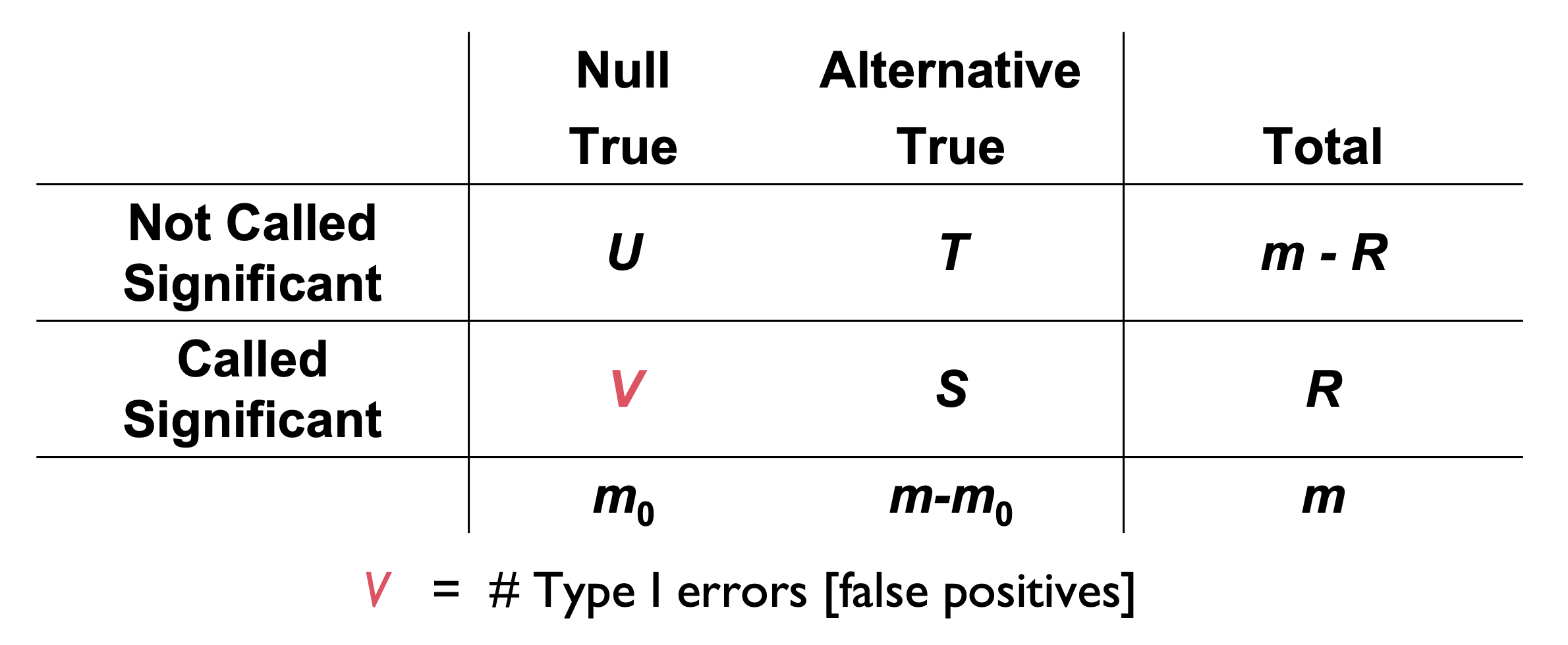
What is the null hypothesis here?
Plot the top 6 probes for genotypeNrlKO
Code
# grab the gene names of the top 6 genes from topTablekeep <-topTable(ebFit, coef ="genotypeNrlKO", number =6) %>%rownames()# extract the data for all 6 genes in tidy formattopSixGenotype <-toLongerMeta(eset) %>%filter(gene %in% keep) %>%mutate(gene =factor(gene, levels = keep))ggplot(topSixGenotype, aes(x = age, y = expression, color = genotype)) +geom_point() +xlab("age (days)") +facet_wrap( ~ gene) +stat_smooth(method="lm", se=FALSE, cex=0.5)
topTable(ebFit, coef = 3) is equivalent here, but much less informative!!
What is the null hypothesis here?
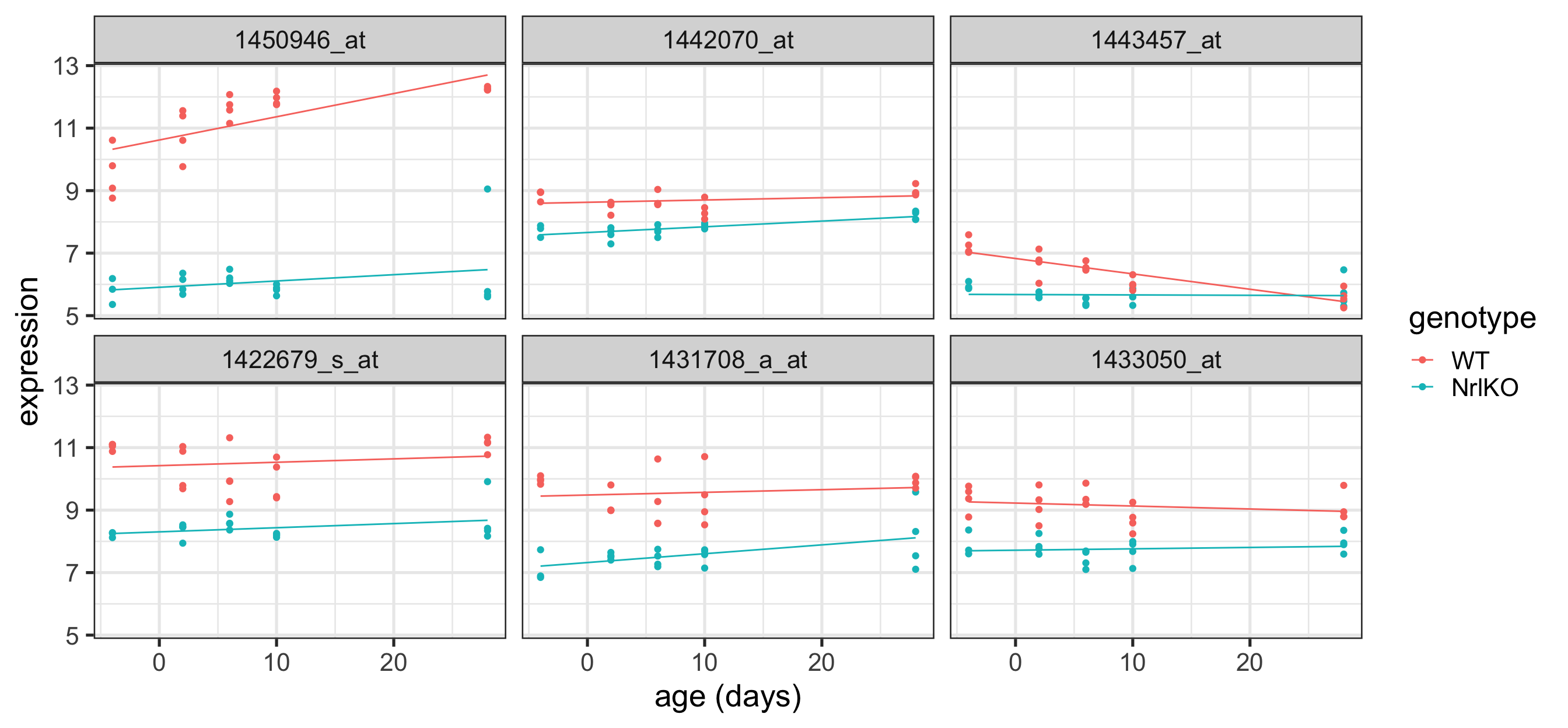
Plot the top 6 probes for age
Code
# grab the gene names of the top 6 genes from topTablekeep <-topTable(ebFit, coef ="age", number =6) %>%rownames()# extract the data for all 6 genes in tidy formattopSixAge <-toLongerMeta(eset) %>%filter(gene %in% keep) %>%mutate(gene =factor(gene, levels = keep))ggplot(topSixAge, aes( x = age, y = expression, color = genotype)) +geom_point() +xlab("age (days)") +facet_wrap( ~ gene) +stat_smooth(method="lm", se=FALSE, cex=0.5)
topTable(ebFit, coef = 4) is equivalent here, but much less informative!!
What is the null hypothesis here?
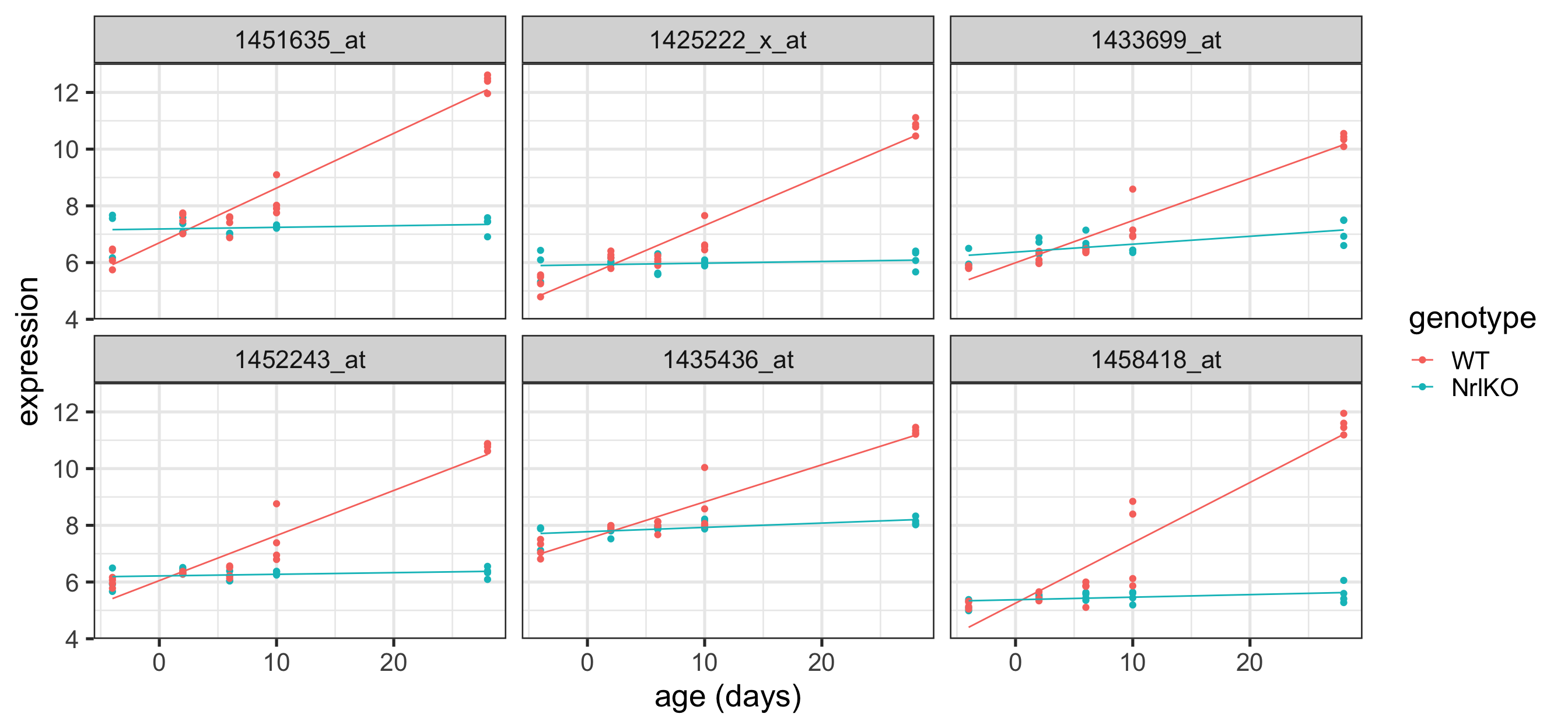
Plot the top 6 probes for genotypeNrlKO:age
Code
# grab the gene names of the top 6 genes from topTablekeep <-topTable(ebFit, coef ="genotypeNrlKO:age", number =6) %>%rownames()# extract the data for all 6 genes in tidy formattopSixItx <-toLongerMeta(eset) %>%filter(gene %in% keep) %>%mutate(gene =factor(gene, levels = keep))ggplot(topSixItx, aes( x = age, y = expression, color = genotype)) +geom_point() +xlab("age (days)") +facet_wrap( ~ gene) +stat_smooth(method="lm", se=FALSE, cex=0.5)
topTable(ebFit, coef = c(2,4)) is equivalent here, but much less informative!!
What is the null hypothesis here?
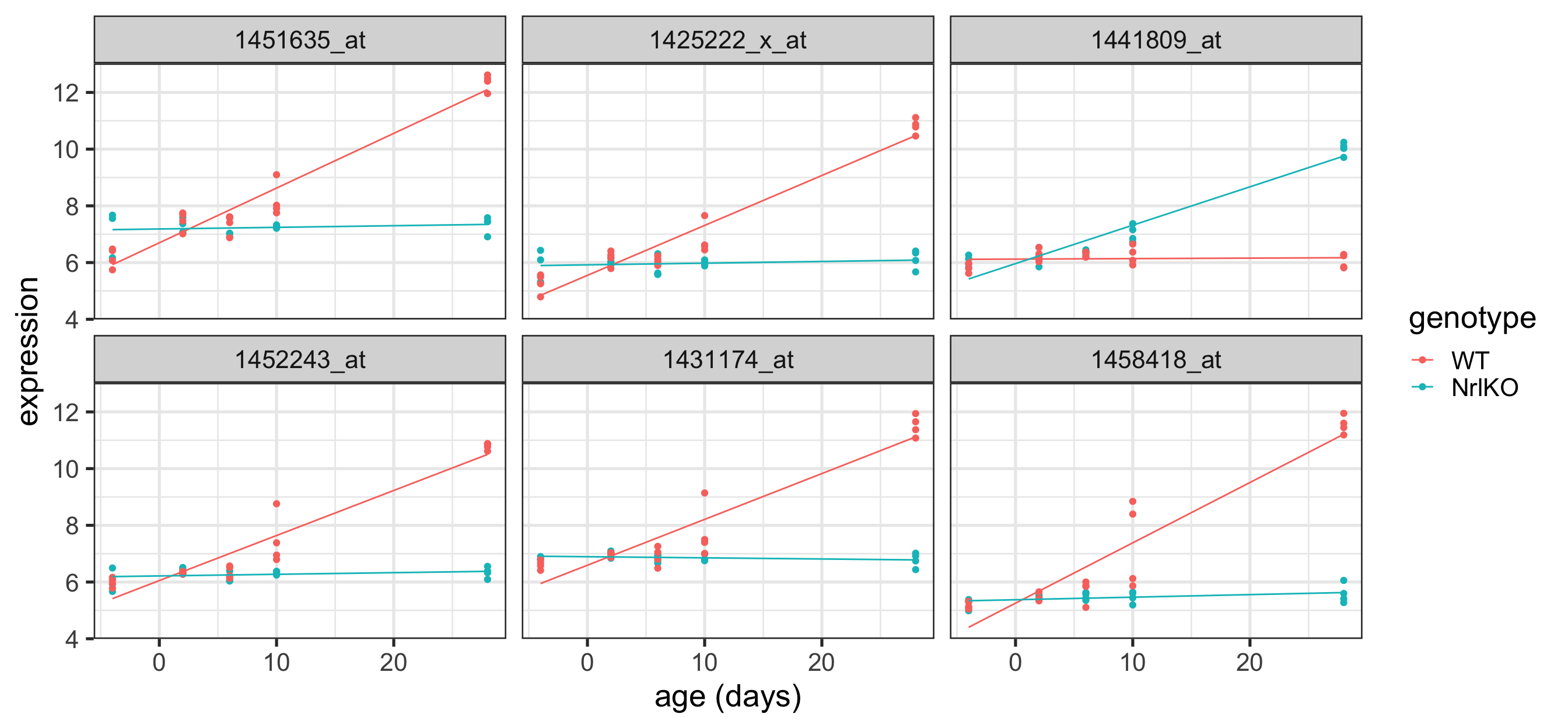
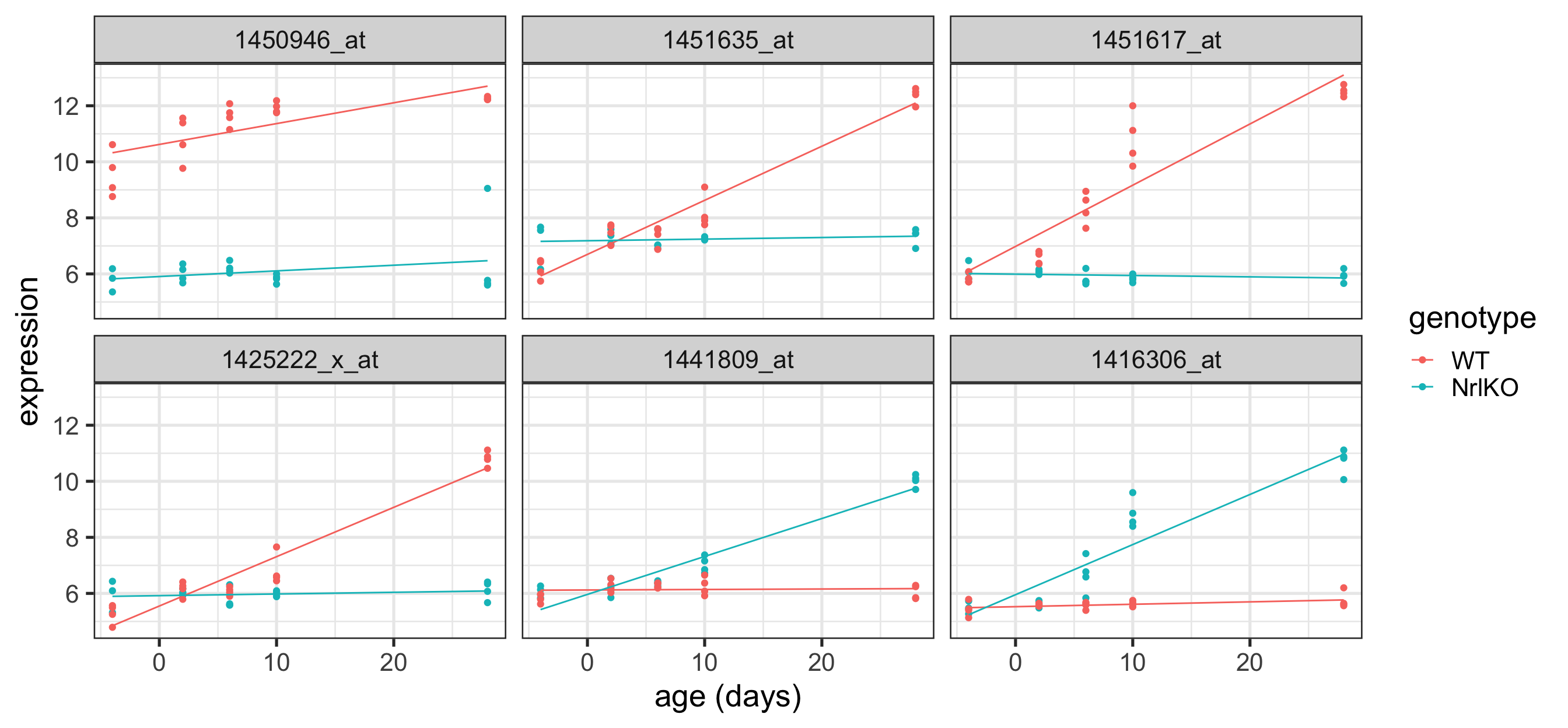
Plot the top 6 probes for any effect of genotype
Code
# grab the gene names of the top 6 genes from topTablekeep <-topTable(ebFit, coef =c("genotypeNrlKO", "genotypeNrlKO:age"), number =6) %>%rownames()# extract the data for all 6 genes in tidy formattopSixGenotypeMarginal <-toLongerMeta(eset) %>%filter(gene %in% keep) %>%mutate(gene =factor(gene, levels = keep))ggplot(topSixGenotypeMarginal, aes( x = age, y = expression, color = genotype)) +geom_point() +xlab("age (days)") +facet_wrap( ~ gene) +stat_smooth(method="lm", se=FALSE, cex=0.5)
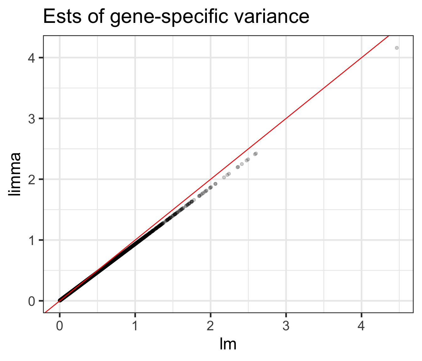
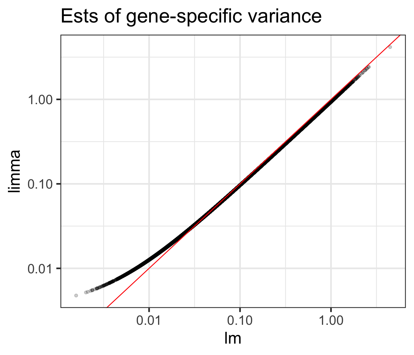
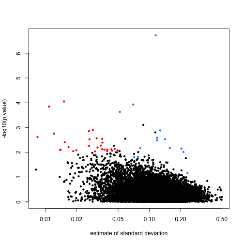
Comparison of \(s_g^2\) and \(\tilde{s}_g^2\) (shrinkage!)
Fill in the blank (increases or decreases):
For large variances, limma ___________ the gene-specific variance estimates.
For small variances, limma ___________ the gene-specific variance estimates.
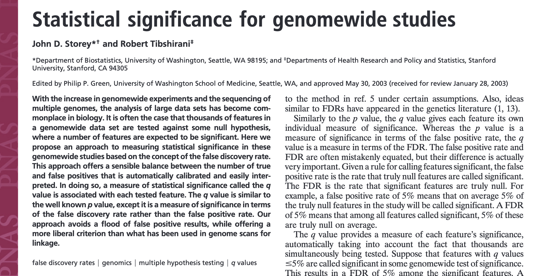
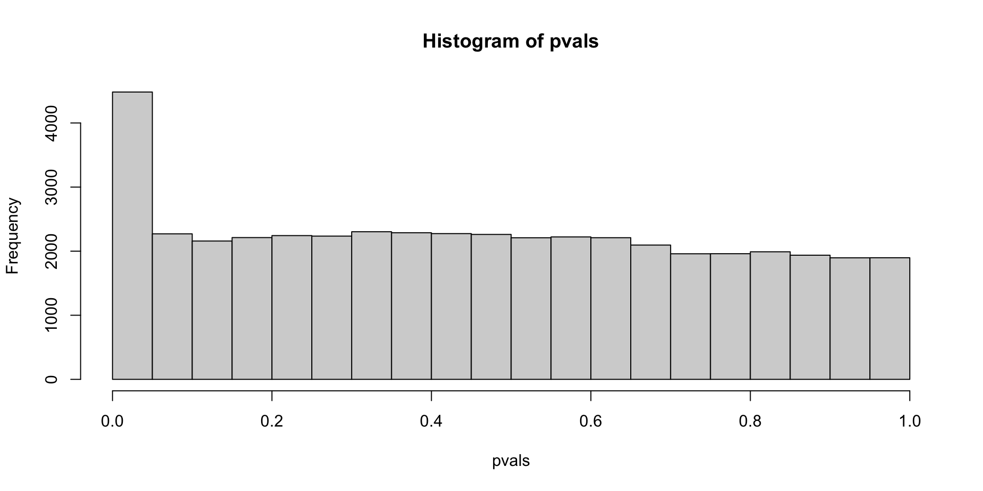
FDR estimates can be invalid (assumptions are violated)
Some possible causes: test assumptions violated, model misspecification, uncontrolled variation/batch effects, selection bias/filtering
Possible solution: nonparametric test
Limitation: lack of flexibility to adjust for multiple covariates
Another possible solution: estimate sampling distribution or p-values “empirically” using resampling techniques
Permutation: construct a simulated version of your dataset that satisfies the null hypothesis and compute statistic (e.g. shuffle group labels for a two-group comparison); repeat many times and use permutation statistics as your sampling distribution rather than a t, Normal, F, \(\chi^2\), etc
Limitation: computationally intensive for genomics; not optimal for small sample sizes
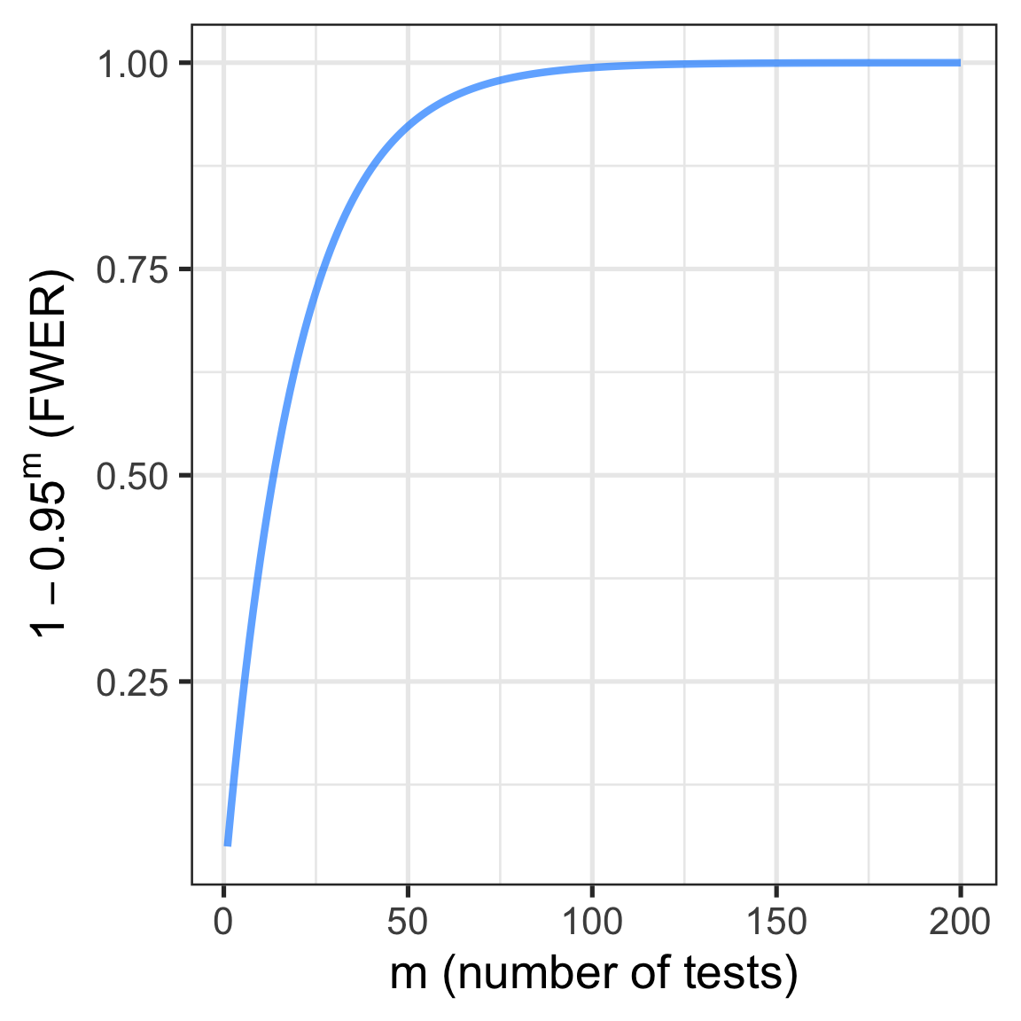
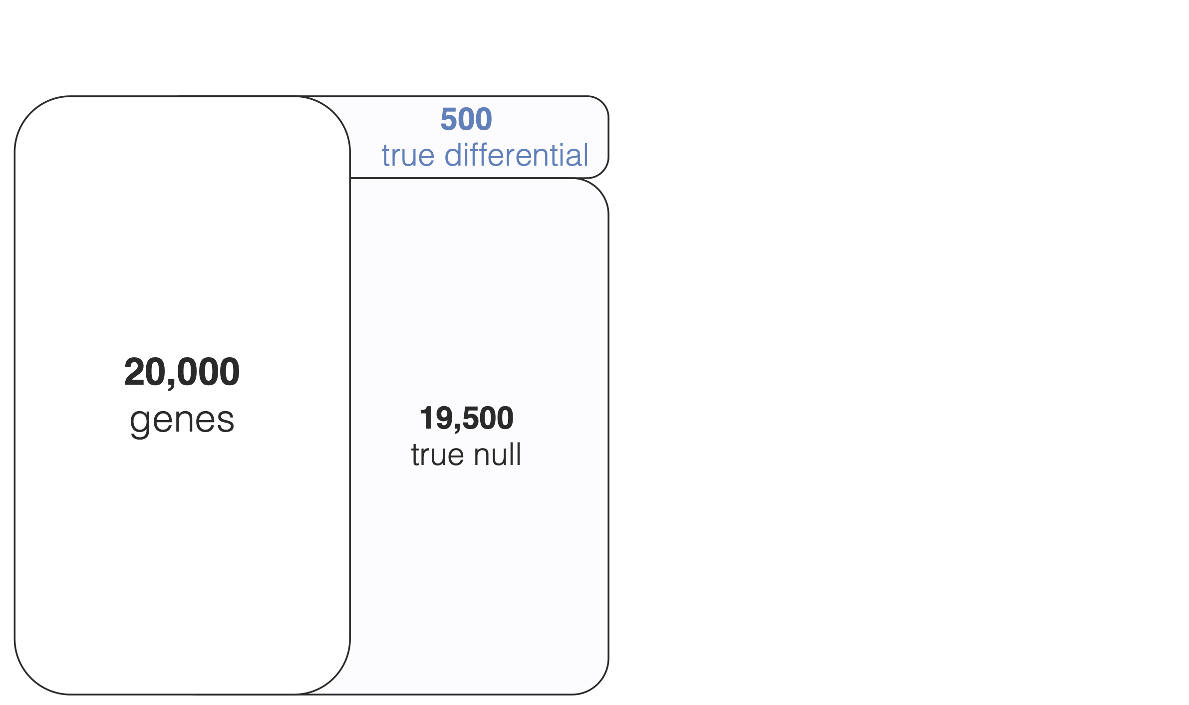
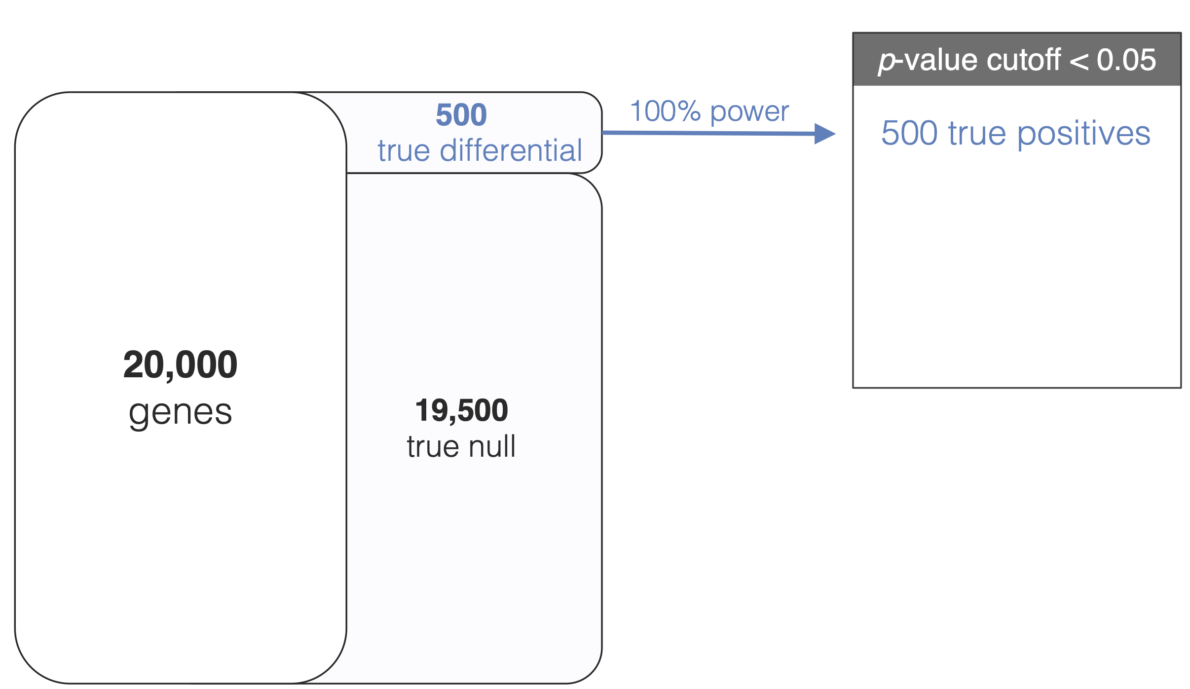
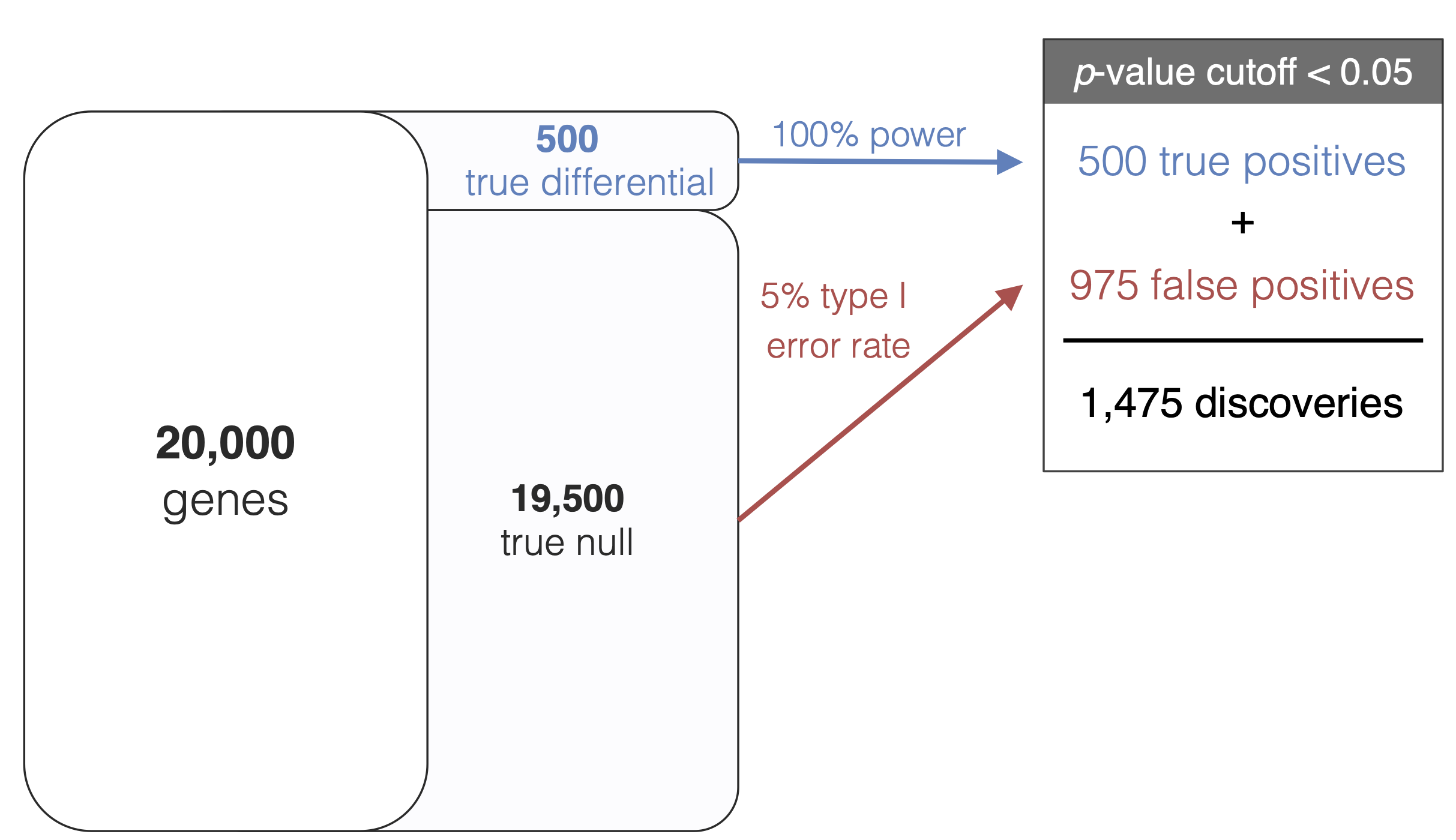
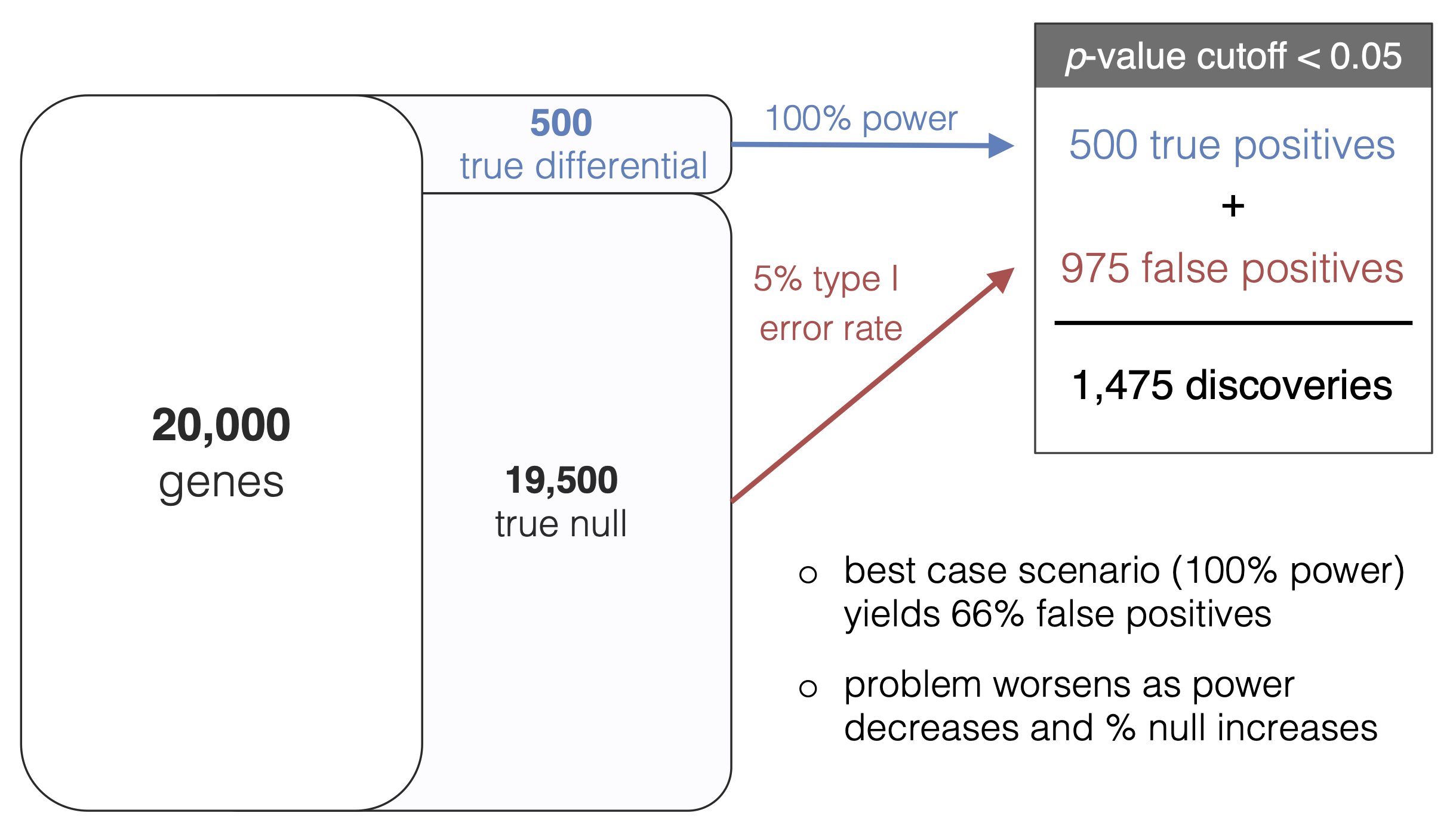
Compounding issues of multiple comparisons
What if you’re not only testing 20K genes, but also multiple tests per gene (e.g. multiple contrasts, such as several two-group comparisons)?
Classical procedures for adjustment (low dimensional setting):
Tukey multiple comparison procedure
Scheffe multiple comparison procedure
Bonferroni or Holm FWER correction
In our setting, we can also apply BH to all p-values globally
limma::decideTests(pvals, method="global") for a matrix of p-values or eBayes output (e.g. rows = genes, columns = contrasts)
p-values are combined, adjusted globally, then separated back out and sorted
Next up: regression with count measures (RNA-seq)!
So far, all of our modeling assumed our outcome \(Y_i\) (gene expression measurements for a particular gene) were continuous and with constant variance (iid).
From RNA-seq, we obtain discrete, skewed distributions (with non-constant variance) of counts that represent gene expression levels across genes. These violate modeling assumptions for standard linear regression / limma.
Next time, we’ll explore:
Data transformations and extensions to limma framework to apply deal with these violations
Generalized linear models (negative binomial regression) to directly model counts