Statistical Inference for RNA-seq

Keegan Korthauer

February 11, 2025

Learning objectives

  • Understand why and when between- and within-sample normalization are needed

  • Apply common between- and within-sample normalization approaches to RNA-seq counts

  • Understand why the count nature of RNA-seq data requires modification to the Differential Expression approaches applied to microarray data (e.g. limma)

  • Apply models such as limma-trend, limma-voom, DESeq2 and edgeR for inference of Differential Expression

A CHD8 RNA-seq experiment

  • Gompers et al. (Nature Neuroscience 2017) analyzed 26 Chd8 mutant and 18 WT mice

    • Tested for differential expression across ~12K genes accounting for sex, developmental stage and sequencing batch
  • We’ll use this dataset throughout this lecture to illustrate RNA-seq analysis

Figures from Gompers et al. (2017) paper

SummarizedExperiment object

SummarizedExperiment: A special object format that is designed to contain (sequencing) data & metadata

Code
# load libraries 
library(tidyverse)
library(limma)
library(DESeq2)
library(edgeR)
library(pheatmap)
library(qvalue)
library(GGally)
library(UpSetR)
library(ComplexHeatmap)
library(TxDb.Mmusculus.UCSC.mm10.knownGene)
library(org.Mm.eg.db)
library(gridExtra)

# Set plotting settings
bcols<-colorRampPalette(c("#000000" ,"#800000" ,"#FF8000" ,"#FFFF00", "#FFFFFF"))(20)
theme_update(panel.grid.major = element_blank(), panel.grid.minor = element_blank())

# read in corrected metadata file
m <- read.csv("data/nn.4592-S4.fixed.csv") %>%
   mutate(Sample = Sample.ID) %>%
   column_to_rownames(var = "Sample.ID") %>%
   dplyr::select(-Number)

# rename variables and recode factor levels 
# for convenience
m <- m %>% 
   dplyr::rename(DPC = `Stage..DPC.`,
                 Sex = `Sex..1.male.`,
                 Group = `Group..1.WT.`,
                 SeqRun = `SeqRun`,
                 MappedReads = `Mapped.Reads`,
                 FeatureCounts = `Feature.Counts`) %>%
   mutate(Sex = factor(Sex, labels = c("M", "F")),
          Group = factor(Group, labels = c("WT", "Mu")),
          SeqRun = factor(SeqRun),
          DPC = factor(DPC))

# read in count matrix
counts <- read.table("data/Gompers_NN_CountMatrix.txt", 
                     header = TRUE, row.names = 1) %>% 
  filter(rowSums(.) > 0)

# place data into SummarizedExperiment object
sumexp <- SummarizedExperiment(assays = SimpleList(counts = as.matrix(counts)), 
                               colData = DataFrame(m))
sumexp
class: SummarizedExperiment 
dim: 20962 44 
metadata(0):
assays(1): counts
rownames(20962): 0610005C13Rik 0610007P14Rik ... Zzef1 Zzz3
rowData names(0):
colnames(44): Sample_ANAN001A Sample_ANAN001B ... Chd8.adult.S29
  Chd8.adult.S31
colData names(7): DPC Sex ... FeatureCounts Sample

Anatomy of a SummarizedExperiment object

A look inside our SummarizedExperiment object

assays(sumexp)$counts %>% head()
              Sample_ANAN001A Sample_ANAN001B Sample_ANAN001C Sample_ANAN001D
0610005C13Rik              20              24              20               8
0610007P14Rik            1714            1796            1970            1996
0610009B22Rik             578             866             790             858
0610009L18Rik              50              82              38              64
0610009O20Rik            2580            2964            2942            3084
0610010B08Rik               0              10               0               2
              Sample_ANAN001E Sample_ANAN001F Sample_ANAN001G Sample_ANAN001H
0610005C13Rik               6              18              17              20
0610007P14Rik            1864            1626            2103            1422
0610009B22Rik             786             662             710             502
0610009L18Rik              70              28              51              44
0610009O20Rik            2848            2640            3210            2160
0610010B08Rik               0               0               3               0
              Chd8.e14.S12 Chd8.e14.S13 Chd8.e14.S14 Chd8.e14.S16 Chd8.e14.S17
0610005C13Rik           16           18           19            8           11
0610007P14Rik          722          974          633          974          914
0610009B22Rik          369          477          402          497          530
0610009L18Rik           41           75           51           57           54
0610009O20Rik         1122         1352          917         1281         1241
0610010B08Rik            0            0            0            0            0
              Chd8.e14.S18 Chd8.e14.S19 Chd8.e14.S20 Chd8.e14.S21
0610005C13Rik            6            6            5            6
0610007P14Rik          908          797          547          908
0610009B22Rik          472          458          282          493
0610009L18Rik           59           62           24           51
0610009O20Rik         1086         1005          723         1289
0610010B08Rik            0            0            0            0
              Chd8.e17.5.1_S158 Chd8.e17.5.2_S159 Chd8.e17.5.4_S161
0610005C13Rik                16                 8                 8
0610007P14Rik              1060               698              1060
0610009B22Rik               283               251               359
0610009L18Rik                25                33                30
0610009O20Rik              1006               519               808
0610010B08Rik                 0                 0                 0
              Chd8.e17.5.5_S162 Chd8.e17.5.6_S163 Chd8.e17.5.1_S1
0610005C13Rik                10                 9              32
0610007P14Rik               779              1142            2530
0610009B22Rik               258               302             566
0610009L18Rik                29                42              77
0610009O20Rik               842               880            2187
0610010B08Rik                 4                 0               0
              Chd8.e17.5.2_S2 Chd8.e17.5.3_S3 Chd8.e17.5.4_S4 Chd8.e17.5.5_S5
0610005C13Rik              18              13              13               9
0610007P14Rik            2048            1789            2081            2790
0610009B22Rik             425             358             384             473
0610009L18Rik              68              51              31              59
0610009O20Rik            1738            1331            1627            2089
0610010B08Rik               0               0               0               0
              Chd8.P0.S1 Chd8.P0.S10 Chd8.P0.S11 Chd8.P0.S2 Chd8.P0.S3
0610005C13Rik         14           9           7          7          5
0610007P14Rik        793         914         793       1007        849
0610009B22Rik        148         175         167        176        166
0610009L18Rik         40          18          28         34         40
0610009O20Rik        962         731         926        840        893
0610010B08Rik          0           0           0          0          1
              Chd8.P0.S4 Chd8.P0.S5 Chd8.P0.S6 Chd8.P0.S7 Chd8.P0.S8 Chd8.P0.S9
0610005C13Rik          2          3          8          9         10          5
0610007P14Rik       1053        982        747        947       1004        719
0610009B22Rik        220        202        157        201        227        154
0610009L18Rik         41         43         35         39         24         27
0610009O20Rik        912        856        896        942       1156        710
0610010B08Rik          0          0          0          0          0          0
              Chd8.adult.S23 Chd8.adult.S24 Chd8.adult.S25 Chd8.adult.S28
0610005C13Rik             14              5              6              5
0610007P14Rik           1554            961            945            976
0610009B22Rik            398            405            333            447
0610009L18Rik             78             65             37             60
0610009O20Rik           1690           1204           1191           1153
0610010B08Rik              0              0              0              0
              Chd8.adult.S29 Chd8.adult.S31
0610005C13Rik              3             16
0610007P14Rik            907            794
0610009B22Rik            302            372
0610009L18Rik             62             70
0610009O20Rik           1174           1007
0610010B08Rik              0              0
colData(sumexp) %>% head()
DataFrame with 6 rows and 7 columns
                     DPC      Sex    Group   SeqRun MappedReads FeatureCounts
                <factor> <factor> <factor> <factor>   <integer>     <integer>
Sample_ANAN001A     12.5        F       Mu        A    42452222      37655856
Sample_ANAN001B     12.5        M       WT        A    54503162      47106938
Sample_ANAN001C     12.5        M       WT        A    44978512      40448118
Sample_ANAN001D     12.5        F       Mu        A    50099336      44993589
Sample_ANAN001E     12.5        F       Mu        A    47163546      41840678
Sample_ANAN001F     12.5        F       WT        A    43893480      39483622
                         Sample
                    <character>
Sample_ANAN001A Sample_ANAN001A
Sample_ANAN001B Sample_ANAN001B
Sample_ANAN001C Sample_ANAN001C
Sample_ANAN001D Sample_ANAN001D
Sample_ANAN001E Sample_ANAN001E
Sample_ANAN001F Sample_ANAN001F

Now we have count data1

  • In the Nrl microarray experiment we worked with continuous microarray values

  • Now we will work with the raw RNA-seq counts (discrete)

  • These counts represent the number of reads mapping to each feature (gene or transcript) - here we have gene counts

  • Seminar 6 explores how to obtain read counts from alignment (BAM or SAM) files

Recall where these counts came from (Lecture 2)

EDA summary (Lecture 3)

  • Experimental design variables:
    • Group (Genotype: Chd8 mutant vs WT)
    • Sex (M vs F, 2 level factor)1
    • DPC (days post conception, 5 level factor)
    • Batch (sequencing run)
  • Notable findings:
    • Batch and DPC are major sources of variation
    • Batch and DPC are confounded
    • One sample is a potential minor outlier
Code
corr <- data.frame(cor(log2(cpm(assays(sumexp)$counts+1))), 
                 row.names = colnames(sumexp)) %>% 
  as.matrix()

set.seed(12)
Heatmap(corr, 
        col = bcols, 
        name = "corr",
        cluster_rows = FALSE, cluster_columns = FALSE, 
        top_annotation = HeatmapAnnotation(Group = m$Group,
                                           Sex = m$Sex,
                                           Batch = m$SeqRun, 
                                           DPC = m$DPC), 
        row_names_gp = gpar(fontsize = 8), 
        column_names_gp = gpar(fontsize = 8))

Differential expression analysis on Chd8 data

  • Main variable of interest: Group (Genotype: Chd8 mutant vs WT)

  • We’d like to fit a model for each gene so we can test for Group effect, and adjust for:

    • Sex (M vs F, 2 level factor)
    • DPC (days post conception, 5 level factor)
  • Using what we learned in previous lectures, we can formulate this model as

\[Y_{i} = \theta + \tau_{\textsf{Mut}}{\color{magenta} x_{i,\textsf{Mut}}} + \tau_{\textsf{F}} {\color{teal}x_{i,\textsf{F}}} + \tau_{\textsf{D14.5}} {\color{blue}x_{i,\textsf{D14.5}}} + \tau_{\textsf{D17.5}} {\color{blue}x_{i,\textsf{D17.5}}} + \tau_{\textsf{D21}} {\color{blue}x_{i,\textsf{D21}}} + \tau_{\textsf{D77}} {\color{blue}x_{i,\textsf{D77}}} + \epsilon_i\]

\[{\color{magenta}x_{i,Mut}} = \bigg\{\begin{array}{l} 1\text{ if } i \text{ is Mutant} \\ 0 \text{ otherwise}\\ \end{array}, \hspace{1em} {\color{teal}x_{i,F}} = \bigg\{\begin{array}{l} 1\text{ if } i \text{ is Female} \\ 0 \text{ otherwise}\\ \end{array}, \hspace{1em}{\color{blue}x_{i,D\#}} = \bigg\{\begin{array}{l} 1\text{ if } i \text{ is DPC#} \\ 0 \text{ otherwise}\\ \end{array}\]

where \(D\# \in \{D14.5, D17.5, D21, D77\}\)

Differential expression analysis on Chd8 data

  • Our model has no interaction terms (though we could add one if we wish)

  • \(p=6\) variables in our model, adding the intercept means 7 parameters to estimate: \(\theta, \tau_{Mut}, \tau_{F}, \tau_{D14.5}, \tau_{D17.5}, \tau_{D21}, \text{ and } \tau_{D77}\)

  • \(n=44\) samples total, so our model has \(n-p-1=44-6-1=37\) degrees of freedom

  • What is the null hypothesis for the test of differential expression between Chd8 Mut and WT using our model?

  • Recall that since this is an additive model, the parameters represent main effects (not conditional)

Design matrix in R

modm <- model.matrix(~ Sex + Group + DPC, data = colData(sumexp))
modm
                  (Intercept) SexF GroupMu DPC14.5 DPC17.5 DPC21 DPC77
Sample_ANAN001A             1    1       1       0       0     0     0
Sample_ANAN001B             1    0       0       0       0     0     0
Sample_ANAN001C             1    0       0       0       0     0     0
Sample_ANAN001D             1    1       1       0       0     0     0
Sample_ANAN001E             1    1       1       0       0     0     0
Sample_ANAN001F             1    1       0       0       0     0     0
Sample_ANAN001G             1    1       1       0       0     0     0
Sample_ANAN001H             1    1       0       0       0     0     0
Chd8.e14.S12                1    0       0       1       0     0     0
Chd8.e14.S13                1    1       0       1       0     0     0
Chd8.e14.S14                1    0       1       1       0     0     0
Chd8.e14.S16                1    1       1       1       0     0     0
Chd8.e14.S17                1    1       0       1       0     0     0
Chd8.e14.S18                1    1       1       1       0     0     0
Chd8.e14.S19                1    1       1       1       0     0     0
Chd8.e14.S20                1    0       1       1       0     0     0
Chd8.e14.S21                1    0       1       1       0     0     0
Chd8.e17.5.1_S158           1    0       1       0       1     0     0
Chd8.e17.5.2_S159           1    0       0       0       1     0     0
Chd8.e17.5.4_S161           1    1       0       0       1     0     0
Chd8.e17.5.5_S162           1    0       1       0       1     0     0
Chd8.e17.5.6_S163           1    0       1       0       1     0     0
Chd8.e17.5.1_S1             1    1       1       0       1     0     0
Chd8.e17.5.2_S2             1    0       1       0       1     0     0
Chd8.e17.5.3_S3             1    1       1       0       1     0     0
Chd8.e17.5.4_S4             1    1       0       0       1     0     0
Chd8.e17.5.5_S5             1    1       1       0       1     0     0
Chd8.P0.S1                  1    1       1       0       0     1     0
Chd8.P0.S10                 1    1       0       0       0     1     0
Chd8.P0.S11                 1    1       0       0       0     1     0
Chd8.P0.S2                  1    1       1       0       0     1     0
Chd8.P0.S3                  1    1       1       0       0     1     0
Chd8.P0.S4                  1    1       1       0       0     1     0
Chd8.P0.S5                  1    1       0       0       0     1     0
Chd8.P0.S6                  1    0       1       0       0     1     0
Chd8.P0.S7                  1    0       1       0       0     1     0
Chd8.P0.S8                  1    1       0       0       0     1     0
Chd8.P0.S9                  1    1       0       0       0     1     0
Chd8.adult.S23              1    0       0       0       0     0     1
Chd8.adult.S24              1    0       1       0       0     0     1
Chd8.adult.S25              1    0       1       0       0     0     1
Chd8.adult.S28              1    0       1       0       0     0     1
Chd8.adult.S29              1    0       0       0       0     0     1
Chd8.adult.S31              1    1       0       0       0     0     1
attr(,"assign")
[1] 0 1 2 3 3 3 3
attr(,"contrasts")
attr(,"contrasts")$Sex
[1] "contr.treatment"

attr(,"contrasts")$Group
[1] "contr.treatment"

attr(,"contrasts")$DPC
[1] "contr.treatment"

Are we ready to fit the model?

Might start with the limma approach on the raw counts, but…

Not so fast - we have to consider additional sources of variation, and check our assumptions!

  • Sequencing depth

  • Gene length & composition

  • Constant variance assumption

Library size (sequencing depth)

  • Library size: Total number of read counts per sample

  • Ideally this would be the same for all samples, but it isn’t

  • Number of reads per sample depends on factors like how many samples were multiplexed and how evenly, cluster density, RNA quality, etc.

Code
hist(colSums(assays(sumexp)$counts)/1e6, main = NULL, 
     xlab = "library size (million total counts)")

Why does library size matter for between-sample comparison?

Read depth variation is a potential source of confounding!

  • We typically want to compare gene counts between samples

  • Intuition: if we sequence one group of samples 2X as much, gene counts in that sample look ~2X as large even if there’s no DE!

  • You may come across (older) literature where data was down-sampled to make library sizes the same (not recommended)

Within-sample comparisons (gene length)

  • Other factors of variation come into play if we also want to compare counts between genes within sample (less common)

  • At the same expression level, longer genes/transcripts have more read counts

How can we make fair between- and within-sample comparisons?

  • Normalized expression units: expression values adjusted for factors like library size, gene length

    • e.g.RPKM/FPKM, TPM, CPM
    • useful for visualization / clustering (usually log scale)
  • Normalization factors: scalar values representing relative library size of each sample

    • e.g. TMM, DESeq size factors
    • useful to include in models of raw counts to adjust for library size
  • For analysis (e.g. DE) it is ideal to start with raw counts

    • raw counts required for many methods
    • can always compute normalized values from raw counts (but not vice versa)

Normalized expression units

  • RPKM/FPKM: reads/fragments per kb of exon per million mapped reads

\(RPKM_{ij} = \frac{R_{ij}}{\frac{L_j}{10^3}\frac{\Sigma_j R_{ij}}{10^6}}\)

For example, if \(R_{ij} = 28\) reads in sample \(i\) for gene \(j\) (which has length \(L_j\) = 2000), and \(\Sigma_j R_{ij} = 11\) million total reads in sample i:

\(RPKM_{ij} = \frac{28}{\frac{2000}{10^3}\frac{1.1\times10^7}{10^6}} = 1.27\)

  • FPKM is the more appropriate term for paired-end data

Normalized expression units, continued

  • TPM: Transcripts per million \[TPM_{ij} = \frac{R_{ij}}{L_j}\frac{10^6}{\Sigma_j R_{ij}/L_j} = \frac{FPKM_{ij}}{\Sigma_j FPKM_{ij}/10^6}\]
  • CPM: Counts per million \[CPM_{ij} = \frac{R_{ij}}{\Sigma_j R_{ij}/10^6}\]
  • See this useful blog post on relationship between these units

  • Which of these measures are between-sample normalization measures? Within-sample? Both?

RNA composition bias

  • Finite number of reads implies that observing reads for one gene decreases ability to observe reads for other genes

  • This isn’t a major problem unless there are large differences in composition between samples, but should be inspected

    • Normalization factors are generally robust to this

Effect of RNA composition bias

Figure source

By CPM or FPKM, genes X, Y, and Z appear less expressed in sample A compared to B

Normalization factors

  • Estimate effective library size, robust to composition bias

  • Not used as a direct data adjustment, but included in a statistical model

  • Example: TMMtrimmed means of M-values (Robinson & Oshlack, 2010)

    • M-values: per-gene ratios of counts among samples
    • Trimmed: extreme values are ignored
    • Values adjusted to have product = 1
    • Assumes that no more than 50% DE
    • Calculate with edgeR::calcNormFactors
Code
dge <- DGEList(assays(sumexp)$counts)
dge <- calcNormFactors(dge)
hist(dge$samples$norm.factors, breaks = 9, main = "", xlab = "TMM normalization factor")

Differential expression: Why we need new methods

  • Goal: accurate p-values for our hypothesis tests

    • Accurate: “Uniform under the null”

    • Properties relied upon for inference from \(t\)-statistics may not hold for count data, even after we ‘normalize’

  • Perhaps most important: Heteroskedasticity and Overdispersion

    • Strong mean-variance relationship expected with count data
      • violation of constant variance assumption of linear models
      • over- or under- shrinkage of genes, depending on variance levels
    • Biological variance over and above binomial sampling variance

Impact of heteroskedasticity

  • OLS: assume all errors have the same variance (within gene)

  • If not true, higher variance observations get less weight in minimization of error than they should (since less precise)

    • Standard errors of parameter estimates will be poor estimates

    • Recall: \(t = \frac{\hat{\beta}}{se(\hat{\beta})}\)

    • …So p-values will also be wrong - in case of positive relationship, too small

Code
praw <- data.frame(mean = log10(rowMeans(as.matrix(counts) + 1)),
                   var = log10(rowVars(as.matrix(counts) + 1))) %>%
  drop_na() %>%
  ggplot(aes(x = mean, y = var)) +
  geom_point(alpha = 0.1) +
  ylab("log10(var)") +
  xlab("log10(mean)") +
  ggtitle("log-scale M-V (Unfiltered, raw)")
praw

Options for DE analysis on counts

  • Summary of the problem: Count data is expected to violate both normality and constant variance assumptions

  • Even microarray data usually has some mean-variance relation!

Possibilities for coping:

  1. Use a non-parametric test (e.g. SAMseq – based on Wilcoxon)

  2. Make adjustments and model as usual

  3. Use a model specific for count data

Make adjustments & model as usual: transformation

  • For microarray data, taking logs is often deemed sufficient to reduce M-V trends

  • We’ll use plots like this which are mean vs \(\sqrt{sd}\) (quarter root variance) instead of mean vs variance (you’ll see why later on)

  • Behaviour of Nrl microarray data set (raw on left, log-tranformed on right):

Chd8 data & effect of log transform

Code
pqrt <- data.frame(mean = (rowMeans(as.matrix(counts))),
           var = sqrt(sqrt(rowVars(as.matrix(counts))))) %>%
  drop_na() %>%
  ggplot(aes(x = mean, y = var)) +
  geom_point(alpha = 0.1) +
  xlab("mean") +
  ylab("sqrt(sd)") +
  geom_smooth(method = "loess", se = FALSE, span = 0.3) +
  ggtitle("M vs Quarter-root V (Unfiltered, raw)")

plqrt <- data.frame(mean = rowMeans(log2(as.matrix(counts)+1)),
           var = sqrt(sqrt(rowVars(log2(as.matrix(counts)+1))))) %>%
  drop_na() %>%
  ggplot(aes(x = mean, y = var)) +
  geom_point(alpha = 0.1) +
  geom_smooth(method = "loess", se = FALSE, span = 0.3) +
  xlab("mean") +
  ylab("sqrt(sd)") +
  ggtitle("M vs Quarter-root V (Unfiltered, log2)") 


grid.arrange(praw, pqrt, plqrt, nrow = 1)

For RNA-seq data, log-transformation doesn’t reliably improve the trends

One option: Voom

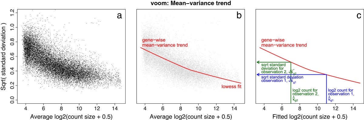
Mean-variance modelling at the observational level

  • Falls under the category “Make adjustments and model as usual”

  • Specifically, adjustment to regular lm to account for M-V relationship + limma

Key ideas of Voom:

  1. heteroskedasticity leads to higher variance observations getting less weight in minimization of error than they should

  2. modeling the mean-variance relationship is more important than getting the probability distribution exactly right (i.e. don’t bother with distributions like Poisson, Binomial, etc that lead to more complicated likelihoods)

Voom implementation

  • Input:

    1. raw counts (required to estimate M-V relationship), but modeling is done on log-transformed CPM values \(((log_2(CPM + 0.5)\) to be precise)

    2. design matrix

  • Output: precision weights and moderated \(t\)-statistics

  • Implemented in limma::voom() function

Voom steps

  1. Fit linear model to \(log_2(CPM_{ig} + 0.5)\) values (samples \(i\)) for each gene \(g\)

  2. Extract the fitted quarter-root error variance estimates \(s^{1/2}_g = \sqrt{sd(\hat{\varepsilon}_{ig}})\)

  3. Fit a smoothed line \(\hat{f}\) to the trend between mean log counts and \(s^{1/2}_g\) using lowess (locally weighted regression)

  1. Use the fitted lowess curve to estimate precision weights: \(w_{ig} = \frac{1}{\hat{f}(\hat{c}_{ig})^4}\) where \(\hat{c}_{ig}\) are the \(log_2\) fitted counts (estimated from model in step 1)

  2. Fit linear model to \(log_2(CPM_{ig} + 0.5)\) values using precision weights \(w_{ig}\)

  3. Compute moderated \(t\)-statistics as before (using eBayes from limma)

Voom illustration

Figure 2, Law et. al, 2014

Why quarter root variance? Details at the end of this slide deck

lowess

  • locally weighted regression fits a smooth curve to approximate the relationship between independent & dependent variables

  • Each smoothed value is given by a weighted linear least squares regression over the span (a neighborhood of the independent variable)

  • Smoothing span is adjustable

  • Generalization to locally weighted polynomial regression & inclusion of multiple independent variables: loess

GIF source: “Intro to Data Science” by Irizarry

How are these ‘precision weights’ actually used in the model?

How can we actually incorporate these precision weights in the regression fit?

Weighted least squares (WLS) regression

  • OLS: \(\boldsymbol{\hat{\beta}}_g = \boldsymbol{(X^TX)^{-1}X^T}\boldsymbol{y}_g\)

  • WLS: \(\boldsymbol{\hat{\beta}}_g = \boldsymbol{(X^T}\boldsymbol{W}_g\boldsymbol{X)^{-1}X^T}\boldsymbol{W}_g\boldsymbol{y}_g\), where \(\boldsymbol{W}_g\) is a diagonal matrix of weights for gene \(g\)

  • Intuition: in minimizing the RSS, we put less weight on data points that are less precise:

\[\boldsymbol{\hat{\beta}}_{g} = argmin_{\beta_{g0}, ..., \beta_{gp}} \Big( \sum_{i=1}^n w_{ig}(\beta_{g0} + x_{i1} \beta_{g1} + ... + x_{ip} \beta_{gp} - y_{ig})^2 \Big)\]

  • Optimal weights to correct for heteroskedasticity: inverse variance1

limma-voom

  • limma-voom is the application of limma to \(log_2(CPM + 0.5)\) values, with inverse variance observational weights estimated from the M-V trend

  • This alleviates the problem of heteroskedasticity and (hopefully) improves estimates of residual standard error

  • Gene-specific variance estimates are ‘shrunken’ to borrow information across all genes:

\[\tilde{s}^2_g = \frac{d_0s_0^2 + ds^2_g}{d_0 + d}\]

  • Note that \(s^2_g\) estimates are affected by voom weights

    • recall that \(s^2_g\) is the sum of squared residuals \(\frac{1}{n-p-1}\hat{\boldsymbol{\epsilon}_g}^T\hat{\boldsymbol{\epsilon}_g}\)
    • under WLS \(\boldsymbol{\hat{\epsilon}}_g = \boldsymbol{y}_g - \boldsymbol{X\hat{\beta}}_g = \boldsymbol{y}_g - \boldsymbol{X(X^T}\boldsymbol{W}_g\boldsymbol{X)^{-1}X^T}\boldsymbol{W}_g\boldsymbol{y}_g\)

limma-voom, continued

  • Moderated \(t\) statistics are then calculated using the shrunken gene-specific variance estimates: \(\tilde{t}_{g} = \frac{\hat{\beta}_{ig}}{\tilde{s}_g \sqrt{v_{ii}}}\)

    • recall that under OLS, \(v_{ii}\) is the \(i^{th}\) diagonal element of \(\boldsymbol{(X^TX)}^{-1}\)
    • under WLS, \(v_{ii}\) is the \(i^{th}\) diagonal element of \((\boldsymbol{X^T}\boldsymbol{W}_g\boldsymbol{X})^{-1}\)
  • Recall:

    • Degrees of freedom for moderated \(t\) statistic: \(n-p-1+d_0\)
    • If \(d_0\) is large compared to \(n-p-1\), moderated statistics have a bigger effect compared to using regular \(t\) statistics (i.e. in general, shrinkage matters more for small sample sizes)

Differential expression analysis on Chd8 data

  • Recall: Our additive model for each gene to test for Group (Chd8 mutant vs WT) effect, and adjust for:

    • Sex (M vs F)

    • DPC (days post conception, 5 levels)

\[Y_{i} = \theta + \tau_{\textsf{Mut}}{\color{magenta} x_{i,\textsf{Mut}}} + \tau_{\textsf{F}} {\color{teal}x_{i,\textsf{F}}} + \tau_{\textsf{D14.5}} {\color{blue}x_{i,\textsf{D14.5}}} + \tau_{\textsf{D17.5}} {\color{blue}x_{i,\textsf{D17.5}}} + \tau_{\textsf{D21}} {\color{blue}x_{i,\textsf{D21}}} + \tau_{\textsf{D77}} {\color{blue}x_{i,\textsf{D77}}} + \epsilon_i\]

\[{\color{magenta}x_{i,Mut}} = \bigg\{\begin{array}{l} 1\text{ if } i \text{ is Mutant} \\ 0 \text{ otherwise}\\ \end{array}, \hspace{1em} {\color{teal}x_{i,F}} = \bigg\{\begin{array}{l} 1\text{ if } i \text{ is Female} \\ 0 \text{ otherwise}\\ \end{array}, \hspace{1em}{\color{blue}x_{i,D\#}} = \bigg\{\begin{array}{l} 1\text{ if } i \text{ is DPC#} \\ 0 \text{ otherwise}\\ \end{array}\]

where \(D\# \in \{D14.5, D17.5, D21, D77\}\)

  • Our model has \(n-p-1=44-7=37\) degrees of freedom

  • We will focus on the null hypothesis of the main effect of Group \(H_0: \tau_{Mut}=0\)

limma-voom in action

# estimate voom weights; plot M-V trend
vw <- voom(assays(sumexp)$counts, 
           design = model.matrix( ~ Sex + Group + DPC, data = colData(sumexp)), 
           plot = TRUE, span = 0.5)  
# run limma with voom weights
lvfit <- lmFit(vw, model.matrix(~ Sex + Group + DPC, data = colData(sumexp)))
lvfit <- eBayes(lvfit)

limma-voom vs limma

Code
# run plain limma (no voom weights) on log cpms
lfit <- lmFit(cpm(assays(sumexp)$counts, prior.count = 0.5, log = TRUE), 
              design = model.matrix( ~ Sex + Group + DPC, data = colData(sumexp)))
lfit <- eBayes(lfit)

# plot moderated t statistics compared to limma-voom
# add dashed lines at x and y intercepts
data.frame(limma = lfit$t[,"GroupMu"], voom = lvfit$t[,"GroupMu"]) %>%
  ggplot(aes(x = limma, y = voom)) +
  geom_hex(bins = 60, aes(fill = stat(log(count)))) +
  geom_abline(intercept = 0, slope = 1) +
  xlab(expression(paste("limma ", tilde(t)[g]))) +
  ylab(expression(paste("limma-voom ", tilde(t)[g]))) +
  geom_vline(xintercept = 0, linetype="dotted") +
  geom_hline(yintercept = 0, linetype="dotted") +
  ggtitle("Moderated t statistics (Chd8 Mu vs WT)")

Another option: limma-trend

Difference between limma-trend and voom

Limma-trend uses the M-V relationship at the gene level, whereas voom uses observational level trends (Law et. al, 2014)

  • Compared to voom, limma-trend treats all observations within a gene the same

  • Compared to regular limma, limma-trend shrinks gene-specific variances toward a global M-V trend, instead of toward a constant pooled variance:

\[\tilde{s}^2_g = \frac{d_0s_{0g}^2 + ds^2_g}{d_0 + d}\]

  • Notice the \(g\) subscript on \(s_{0g}^2\)! The prior variance is different for each gene (unlike in regular limma)

  • Based on the M-V trend, \(s_{0g}^2\) is (typically) higher for lowly expressed genes

limma-trend vs voom?

Figure 2, Law et. al, 2014

Intuition

  • limma obtains one overall prior variance for all genes
  • limma-trend obtains a prior variance for each gene based on it’s mean using a smoothed curve of the mean vs variance
  • limma-voom obtains a weight for each observation from such a curve

limma-trend in action

mm <- model.matrix(~ Sex + Group + DPC, 
                   data = colData(sumexp))
ltfit <- lmFit(cpm(assays(sumexp)$counts, 
                   log = TRUE), 
               design =  mm)
ltfit <- eBayes(ltfit, trend = TRUE)

# limma-trend s^2_{0g}
str(ltfit$s2.prior)
 Named num [1:12158] 0.0287 0.051 0.0274 0.023 0.0268 ...
 - attr(*, "names")= chr [1:12158] "0610007P14Rik" "0610009B22Rik" "0610009O20Rik" "0610010F05Rik" ...
# regular limma s^2_0
str(lfit$s2.prior)
 num 0.0337
Code
# plot histogram of limma trend gene-specific prior variances vs limma prior
data.frame(prior = ltfit$s2.prior) %>% 
  ggplot() + 
  geom_histogram(aes(prior), bins = 35) + 
  scale_x_log10() +
  geom_vline(xintercept = lfit$s2.prior, colour = "red") + 
  geom_text(aes(x = 0.052, y = 3000, label = "limma s_0^2"), colour = "red") +
  xlab(expression(paste("limma-trend ", s["0g"]^2))) +
  ggtitle(expression(paste("limma-trend ", s["0g"]^2, " vs limma ", s[0]^2))) 

Variance-stabilizing transformation (VST)

Another option to account for the Mean-Variance relationship is to apply the VST (Anders & Huber 2010 and implemented in DESeq2):

  • estimates mean-variance relationship and transforms the data to remove (flatten) the experiment-wide trend
  • also accounts for library size differences (like normalization factors)
  • great option for visualization
Code
library("vsn")
meanSdPlot(vst(as.matrix(counts)), 
           ranks = FALSE)

Alternative option: use count models

  • Number of reads observed for gene \(g\) in a given sample is a random variable

  • Say RNA for gene \(g\) is present “in the cell” at about 1 out of every 1,000,000 molecules

    • Abundance \(q_g=1/1,000,000 = 1\times10^{-6}\) (“probability of success”)
  • If we randomly pick \(N = \Sigma_gy_{g} = 1,000,000\) molecules (“reads” = “trials”), how many gene \(g\) RNAs do we expect to see? \(E(y_{g} | N) = \,\, ?\)

  • But could get 0, 2, 3, 4, … etc just by chance: this is a Binomial distribution

Statistics of counts: Binomial and Poisson

  • Binomial probability distribution models the number of successes in \(N\) trials, each with probability of success \(q\) is \((Binomial(N,q))\)
    • mean = \(Nq\)
    • our example: \(y_{g} \sim Binomial(1\times10^{6}, 1\times10^{-6})\)
  • Poisson distribution counts discrete occurrences along a continuous interval of time/space
    • parameterized by a rate parameter \(\lambda\)
    • key difference from Binomial: number of events can be infinitely large
  • For count data, the variance is a function of the mean (very different from a normal)
    • Binomial: mean \(= Nq\), variance \(=Nq(1-q)\)
    • Poisson: mean = variance = \(\lambda\)

Binomial approximation of Poisson

For \(y \sim Binom(N,q)\), if \(N\) is large and \(Nq\) is small (rule of thumb: \(N\) > 20 & \(Nq\) < 5), then

\[\textsf{Approximately } y \sim Poisson(Nq)\]

Poisson approximation in RNA-seq: Overdisperson

Poisson OK for technical replicates, but does not capture biological variability

Negative Binomial distribution to the rescue!

  • Negative Binomial (NB) is also known as a Poisson-Gamma mixture

    • i.e. A Poisson with a rate parameter that is Gamma-distributed (instead of fixed)

    • The Gamma distribution on means captures the biological variance (overdispersion) that can’t be accommodated by Poisson alone

  • “Overdispersed Poisson” (variance \(>\) mean)

  • Key problem: estimating (gene-specific) dispersion from small datasets is tricky!

Negative Binomial GLM

  • Gene-specific variance under NB: \(\sigma_g^2 = \mu_g + \mu_g^2\phi_g\)

    • \(\phi_g\) is the dispersion for gene \(g\)

    • if \(\phi_g=0\), get Poisson!

  • We can perform inference about \(\mu_g\) using GLM: \(E(\boldsymbol{Y|X})=g(\boldsymbol\mu) = \boldsymbol{X\beta}\)

    • using likelihood ratio tests (analogous to F-tests in ANOVA/OLS)

    • using Wald tests for individual coefficients (analogous to t-test in OLS)

  • To do so, we need to treat \(\phi_g\) as known (so first need to estimate it)

Important

Estimation of dispersion is the main issue addressed by methods like edgeR and DEseq2

Disperson estimation

  • One option is to assume \(\phi_g\) is a set parametric function of the mean \(\mu_g\) (e.g. quadratic)

  • More flexible approach is to use empirical Bayes techniques: dispersion is gene-specific but moderated toward the observed trend with the mean

source: Statistical Analysis of Next Generation Sequencing Data, by Chen et al.

DESeq2 vs edgeR

  • These methods are very similar overall

  • Major differences between the methods lie in how they filter low-count genes, estimate normalization factors, estimate prior degrees of freedom, deal with outliers in dispersion estimation, and moderate dispersion of genes with high within-group variance or low counts

    • Also slight differences in specific types of hypothesis tests (quasi-likelihood in edgeR and Wald test in DESeq2)
  • Many of these choices can be altered by changing default parameter settings in both methods (see user manuals)

edgeR in action

des <- model.matrix(~ Sex + Group + DPC, data = colData(sumexp))
dge <- DGEList(counts = assays(sumexp)$counts, 
               samples = colData(sumexp))
dge <- calcNormFactors(dge)
dge <- estimateDisp(dge)
QLfit <- glmQLFit(dge, design = des)
QLtest_Group <- glmQLFTest(QLfit, coef = "GroupMu") 

topTags(QLtest_Group)
Coefficient:  GroupMu 
             logFC   logCPM         F       PValue          FDR
Chd8    -0.5910169 7.168410 136.93350 1.060551e-14 1.289418e-10
Dnajc4   0.3318225 3.483504  45.44089 3.682335e-08 2.238491e-04
Vrk3     0.2278501 5.018357  40.30631 1.334186e-07 5.407010e-04
Hmgcll1 -0.2725199 4.679259  33.17377 9.253342e-07 2.463745e-03
Gh      -1.0930426 4.327084  35.11644 1.013220e-06 2.463745e-03
Xrcc4    0.3206540 3.800252  31.97145 1.307488e-06 2.649407e-03
Myef2   -0.2631618 6.465549  29.11564 3.045538e-06 4.068467e-03
Lrrc48   0.4081822 3.078380  28.94894 3.204690e-06 4.068467e-03
Usp11   -0.2680673 7.332344  28.89415 3.256932e-06 4.068467e-03
Anxa11   0.4735432 2.957357  28.47633 3.716860e-06 4.068467e-03

DESeq2 in action

des <- model.matrix(~ Sex + Group + DPC, data = colData(sumexp))
dds <- DESeqDataSet(sumexp, design = des)
dds <- estimateSizeFactors(dds)
dds <- DESeq(dds)

res <- results(dds, name = "GroupMu")
res[order(res$padj), ]
log2 fold change (MLE): GroupMu 
Wald test p-value: GroupMu 
DataFrame with 12158 rows and 6 columns
         baseMean log2FoldChange     lfcSE      stat      pvalue        padj
        <numeric>      <numeric> <numeric> <numeric>   <numeric>   <numeric>
Chd8     3559.907      -0.595924 0.0531048 -11.22165 3.19249e-29 3.80513e-25
Dnajc4    276.096       0.334895 0.0512012   6.54076 6.12065e-11 3.64760e-07
Vrk3      799.700       0.217710 0.0345255   6.30578 2.86745e-10 1.13924e-06
Hmgcll1   633.353      -0.279578 0.0494532  -5.65339 1.57318e-08 4.68767e-05
Anxa11    194.990       0.514626 0.0930202   5.53241 3.15858e-08 7.52943e-05
...           ...            ...       ...       ...         ...         ...
Wdr52    113.6225     -0.3634976 0.1600699 -2.270868   0.0231550          NA
Wisp1     88.5170      0.3151848 0.1661647  1.896822   0.0578514          NA
Wnt10a    85.9890      0.2485353 0.2584913  0.961484   0.3363089          NA
Wnt5b    110.0166      0.0966134 0.0960656  1.005703   0.3145585          NA
Xdh       46.8604      0.5709232 0.2895838  1.971530   0.0486632          NA

A note on ‘Contrasts’

Let’s say we want to test a combination of coefficients being equal to zero, like DPC 77 vs 21

Contrasts are a linear combination of parameters where the weights add up to zero

They allow you to carry out a specific comparison between different groups within your experimental design.

resultsNames(dds)
[1] "Intercept" "SexF"      "GroupMu"   "DPC14.5"   "DPC17.5"   "DPC21"    
[7] "DPC77"    
results(dds, contrast = c(0, 0, 0, 0, 0, -1, 1))
log2 fold change (MLE): 0,0,0,0,0,-1,+1 
Wald test p-value: 0,0,0,0,0,-1,+1 
DataFrame with 12158 rows and 6 columns
               baseMean log2FoldChange     lfcSE       stat      pvalue
              <numeric>      <numeric> <numeric>  <numeric>   <numeric>
0610007P14Rik  1135.170     -0.0710865 0.0941651  -0.754913 4.50301e-01
0610009B22Rik   374.752      0.7433605 0.1312935   5.661822 1.49774e-08
0610009O20Rik  1286.616      0.1521567 0.0609685   2.495662 1.25722e-02
0610010F05Rik  3606.866     -1.3149332 0.0809749 -16.238766 2.68267e-59
0610010K14Rik  1415.398     -1.0341080 0.1043641  -9.908656 3.81747e-23
...                 ...            ...       ...        ...         ...
Zxdc            889.692      0.0299690 0.0615856   0.486624   0.6265251
Zyg11b         7063.757     -0.1567778 0.0993863  -1.577459   0.1146900
Zyx            1835.530     -0.0293001 0.0884080  -0.331420   0.7403276
Zzef1          1584.677      0.2220581 0.1195990   1.856689   0.0633554
Zzz3           2216.782     -0.0237226 0.0598424  -0.396418   0.6917964
                     padj
                <numeric>
0610007P14Rik 4.86226e-01
0610009B22Rik 3.01433e-08
0610009O20Rik 1.64729e-02
0610010F05Rik 5.50763e-58
0610010K14Rik 1.74427e-22
...                   ...
Zxdc            0.6584907
Zyg11b          0.1354262
Zyx             0.7657263
Zzef1           0.0772338
Zzz3            0.7205497

We can do this in limma, edgeR and DESeq2

How to choose a method?

Example comparison 1: Love et al. (2018)

Example comparison 2 (for single-cell RNA-seq)

Soneson & Robinson (2018)

How to choose a method?

  • No established gold standards

    • Simulations somewhat unsatisfying (depend on specific settings)

    • In real data, the truth is unknown

The most popular and widely used methods tend to give similar results

  • edgeR and DESeq2 are very similar in design

    • typically expected to work better for small sample sizes or low read depth
  • limma-trend or limma-voom also sound choices

    • work equally well when library sizes don’t vary much

    • might not do as well when sample size or depth is very low (data is more discrete)

Comparing methods on the Chd8 dataset

tl;dr version: there isn’t a big difference

Possible reasons why:

  • methods have been converging in approach

  • modeling count data directly with GLMs is more important for smaller samples sizes, lower read depth

Check out the comparisons in detail (including the results of edgeR and DESeq2 in the companion notes

Rank correlation of p-values for effect of Chd8 mutation

Heatmap of top 30 genes by limma-trend, adjusted for DPC effect

Additional resources

  • Chapter 1: Generative Models for Discrete Data in Modern Statistics for Modern Biology by Holmes and Huber is a great review of count models

  • Detailed comparison of these methods on the Chd8 dataset can be found here

  • For all of the specific methods we discuss, refer to the Bioconductor pages (vignettes, reference manuals) for the most current and thorough details on implementation

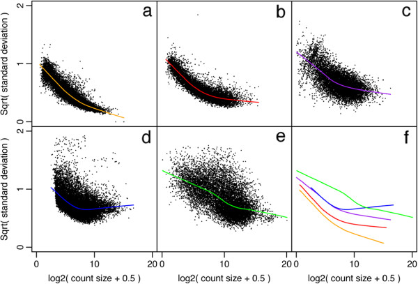
Aside: Why quarter-root variance?

  • The coefficient of variation \((CV = \frac{\sigma}{\mu})\) for RNA-seq counts is roughly \(\sqrt{\frac{1}{\lambda} + \phi}\)

    • \(\lambda:\) expected size of count; arises from technical variability associated with sequencing and gradually decreases with increasing count size

    • \(\phi:\) measure of biological variation (overdispersion); roughly constant

  • Standard deviation of \(log_2(CPM)\) is approximately equal to CV of the counts (by Taylor’s theorem)

\[sd(log_2(CPM)) \approx \sqrt{\frac{1}{\lambda} + \phi}\]

Back

Why quarter-root variance?

Note

Coefficient of variation (CV) of RNA-seq counts should be a decreasing function of count size for small to moderate counts, and asymptote to a value that depends on biological variability

Law et al. 2014: Panels (a)-(e) represent datasets with increasing expected biological variability

Square root of standard deviation used as distribution is more symmetric (i.e. less skewed)